Plots and Graphs on the TI-83

Chapter 3 in the text starts with a display of the calculator screen. It may not be the case that your calculator looks like the figure given in the text. The purpose of this page is to both construct the display and to learn how to get rid of or to hide that display. After that, this page constructs the two graphs given at the top of page 121 in the text.

Figures 1-8: demonstrate methods for clearing one list, many lists, and all lists.
Figures 9-10: set up the list editor, i.e., place the default lists into the list editor.
Figures 11-15: insert the values used in the text into two lists, L1 and L2.
Figures 16-17: remove any residual function definitions.
Figures 18-19: set the ZDecimal ZOOM attributes and show a blank graph.
Figures 20-23: set up the initial plot and show the graph.
Figures 24-26: finally produce the plot that appears in the text.
Figures 27-28: demonstrate the TRACE feature for plotted points.
Figures 29-31: demonstrate adjusting the Xscl value to "clean up" the plot.
Figures 32-34: show the steps to turn off a plot of points.
Figures 35-40: produce the graph shown on the left and at the top of page 121 in the text.
Figures 41-45: produce the graph shown on the right and at the top of page 121 in the text.

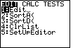
Figure 1	We will start with the calculator showing the STAT menu by pressing the key. This screen shows the options that are available. In fact, there are three sub-menus to the STAT menu, namely, EDIT, CALC, and TESTS. These are listed across the top of the screen. As noted by the highlight of EDIT at the top of the screen, we are are seeing, in Figure 1, the EDIT sub-menu.
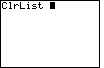
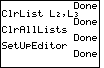
Figure 2	The first thing that we want to do is to clear out some of the lists that may have values in them on your calculator. To do this we can use the number 4 option on the screen, ClrList. We could move the highlight down to is item and press the ENTER key, or we could just press the key. The result is shown in Figure 2. All that has been done is to paste the command ClrList onto the screen.
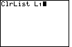
Figure 3	The TI-83 has six built-in lists, L1 through L6. We will start by creating a command that will reset the L1 list. To do this we need to add L1 to the command. We use the keys to place L1 onto the screen. This is reflected in Figure 3. Now that the command is formed, we press the key to perform the command. The result, shown in Figure 4, is that the calculator responds with Done.
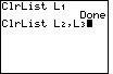
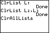
Figure 4	The ClrList command can reset more han one list. In fact we can clear multiple lists by placing the names of the lists after the command, but separated by commas. Thus, to clear lists L2 and L2 we can recall the previous command, via , then backspace over the L1 by pressing , and then using the keys to generate the names. The result is shown in Figure 4.
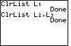
Figure 5	Again, with the command formed in Figure 4, we ask the calculator to perform the command by pressing the key. The calculator responds with Done, as shown in Figure 5.
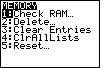
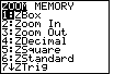
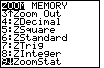
Figure 6	While the ClrList command can be used to clear individual lists, or to clear a series of lists, there is a command on the TI-83 to clear all lists. That command is in the MEM menu. We open that menu via the keys. The menu is shown in Figure 6. Within that MEM menu, item 4, ClrAllLists, is the command that we can use to reset all lists. We select that option by pressing the key. This will paste the ClrAllLists command onto the screen, as shown in Figure 7.
Figure 7	Again, to perform the command, we press the key.
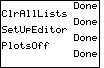
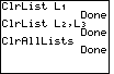
Figure 8	Figure 8 shows the calculator response, Done. All lists have been reset.
Figure 9	In Figure 9 we return to the STAT menu, via the key. This time we want to use option 5, SetUpEditor. To do this we press the key.
Figure 10	The SetUpEditor command is used to put certain lists into the list editor. If used by itself, as we have in Figure 10, the command automatically places L1 through L6 into the editor. We perform the command by pressing the key, and the calculator responds with the usual Done.
Figure 11	Our next step will be to edit L1 and L2 to hold certain values. In particular, we want the ordered pairs (-40,4), (-2,2), (0,0), (2,2), and (4,4) placed into the system. We will enter the x-values into L1 and the y-values into L1. We get back to the STAT menu via the key. Figure 11 shows that menu. We want to edit the lists that we have just placed into the list editor. Therefore, we press to select the already highlighted Edit option.
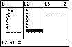
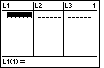
Figure 12	Figure 12 shows the first three lists, L1 L2 and L3 that are in the list editor (L4, L5, and L6 are in the editor but are note shown). Each of the lists is empty, which is what we expect having given the ClrAllLists command back in Figure 8. The highlight is on the place in L1 where the first value could be entered. Furthermore, at the bottom of the display, we note that the calculator is waiting for a value to be placed into L1(1)
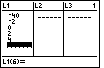
Figure 13	We produce Figure 13 by entering the required values for the first list. The keystrokes needed to do this are .
Figure 14	Now that the values are entered into L1 we can press the key to move the highlight to the L2 list. This is shown in Figure 14.
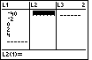
Figure 15	We use to produce the second set of values in this second list. Now that all of the values are in the lists, and before we move to see the plot of the points defined by these two lists, let us set up some of the other components.
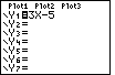
Figure 16	First, we will make sure that we do not have any graph functions defined. To do this we press the key. This will display a screen that should be similar to the one shown in Figure 16. The calculator used to generate Figure 16 has one graph function defined already, namely, Y1=3X-5. We want to remove that function. The highlight is on that function, in the form of a blinking cursor over the "3". Therefore, we can completely remove the graph function by pressing the key.
Figure 17	Figure 17 shows the result of clearing the graph function in Figure 16. At this point we can move to the ZOOM screen to set the parameters for the graph window. We do this by pressing the key. This will move us to the display shown in Figure 18.
Figure 18	The first three options in the menu have more to do with our normal, everyday understanding of ZOOM. ZBOX lets us draw a box around an area of a graph and, when we are done, have the calculator focus in on that boxed region. ZIN and ZOUT allow us to zoom in and zoom out either toward a point or away from a point on the graph. The reminaing items on Figure 18 do not behave with our usual understanding of ZOOM. For example, ZDECIMAL is used to set the window parameters of a graph so that each point on the graph is centered on a standard decimal value. We will use the ZDECIMAL option by pressing the key. This will set the parameters and it will move us to the graph screen, shown in Figure 19.
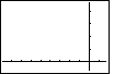
Figure 19	Given the steps we have taken, the axes on your calculator should look identical to those in Figure 19. It is possible that you have three of our points plotted on your graph and that the graph looks more like Figure 23. If your screen does look like Figure 23 then your calculator is already set to plot L1 and L2. The calculator used to generate Figure 19 was not set to plot anything. We will need to turn on the plot for the points specified in L1 and L2. To do this we need to move to the STAT PLOT menu via the keystrokes .
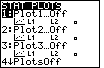
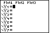
Figure 20	Figure 20 shows the STAT PLOT menu. The TI-83 can plot three separate sets of pairs of values. The names Plot1, Plott2, and Plot3 identify these three different plots. The STAT PLOT menu shown in Figure 20 merely gives the status of all three plots, along with the option (4:PlotsOff) of turning off all of them. Off the screen, there is an optionto turn on all three plots (5:PlotsOn). We are interested in turning on Plot1. The STAT PLOT menu merely reports the status of Plot1. To turn it on we select the first option, which is already highlighted, by pressing the .
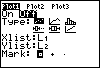
Figure 21	Figure 21 shows the resulting detail for Plot1. On this screen we can turn the plot On or Off, we can set the type of the plot, we can select the two lists to use (one to hold the x-values and one to hold the y-values), ans we can choose the kind of "marker" to be used to plot the points. All we want to do is to turn On the plot. We note that the Off option is currently selected. However, not shown in Figure 21, the cursor will be blinking over the On option. We select that On option by pressing the .
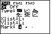
Figure 22	Figure 22 shows the change in the menu. Plot1 is now turned On. In addition, Plot1 is already using L1 for the Xlist and L2 for the Ylist. If this were not the case, then we would have to change these two settings. We are done modifying the settings. We return to the graph by pressing the key.
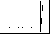
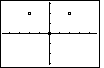
Figure 23	Now, in Figure 23, we can start to see the points that we entered way back in Figures 11 through 15. The problem is that we are only seeing three of the points. The screen parameters were set by the ZDecimal option. Therefore, the x-axis extendes from -4.7 to 4.7 and the y-axis extends from -3.1 to 3.1. Two of our points fall out of this field, namely (-40,4) and (4,4). Therefore, those two points are not plotted on the screen.
Figure 24	We return to the ZOOM menu, by pressing the key. We are going to use this menu to change the window settings. We do this because the TI-83 has an option that will set the parameters according to the values in the lists to be plotted. The option we want is ZoomStat, but it is not shown on the initial ZOOM menu shown in Figure 24. We will have to move down the menu to uncover some more options. We press the key 8 times to move to Figure 25.
Figure 25	Now we hav highlighted the ZoomStat option. As noted, this option will readjust the graph parameters so that all of the points specified by the two lists will be on the graph. We select the ZoomStat option and move back to the graph window by pressing the key.
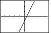
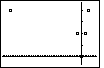
Figure 26	Figure 26 has the modified graph. This graph is identidal to the one in the text on page 126. Rather than stop here we will take this opportunity to demonstrate a little more about this plot. First, we will press the key to move into TRACE mode.
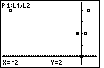
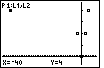
Figure 27	In TRACE mode, the TI-83 diplays, at the upper left of the screen what we are tracing. In this case, we are tracing the points in Plot1 and they come from the lists L1 and L2. Therefore, the upper left of the screen in Figure 27 shows P1:L1,L2. TRACE mode also highlights a point on the list and gives its coordinates at the bottom of the screen. In Figure 27 the first point is highlighted and its coordinates, X=-40 and Y=4 are given at the bottom. We can move to the next point by pressing the key.
Figure 28	In Figure 28 we have moved to highlight the second point. Again, its coordinates are given at the bottom of the TRACE screen. by using the left and right cursor keys we can move through all of the points in Plot1. One of the ugly parts of the graph that we have is the heavy concentration of "tick" marks on the X-axis. There is a tick mark for every X-value from -44 to 8. We can see the reason for this, and change it, by looking in the WINDOW menu. We move to that menu by pressing the key.
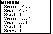
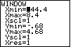
Figure 29	The WINDOW screen shows us the limits on the X and Y values for a graph, as well as the frequency with which the "tick" marks are placed on the graph. From Figure 29 we see that the X-values do in fact range from -44.4 to 9.4 and the Y-values from -0.68 to 4.68. The Xscl value in Figure 29 is 1. Thus, there is a tick mark for every integer value of X. The leftmost tick mark will be at -44 and the rightmost at 8. Thus, there are 53 tick marks across a screen that has all of 95 pixels. As a result, as we can see in Figure 28, over half of the pixels just above the X-axis are turned on as tick marks.
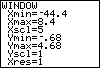
Figure 30	We can change the frequency of the tick marks by changing the value assigned to Xscl. We do this by moving the highlight down, using the key twice, to highlight the Xscl value, and then pressing the keys for the desired new value. In Figure 30 we have pressed the to set the Xscl to 5. We can return to the Graph window by pressing the key. This will produce Figure 31.
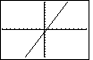
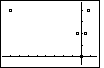
Figure 31	THe plot in Figure 31 is identical to our earlier plot, Figure 26, except that we now have tick marks on the X-axis at every fifth integer, -40, -35, -30, ...

The textbook moves from this display to a graph of the function y=2x-1, at the top of page 128. We will to look at the steps needed to make this transformation.

Figure 32 The plot that we developed above needs to be turned off. If we were to leave it on we would keep getting the points stored in our two lists, L1 and L2, displayed on our graphs. We return to the STAT PLOT menu to turn off the plots. The keystokes to open the menus are . This produces the menu shown in Figure 32. Note that Plot1 is marked as On in Figure 32. We could go into the submenu for Plot1 and turn it off there. However, we also have option 4 on the screen, PlotsOff, which will turn off all three of the plots. We will opt for this method, and we press to select it.

Figure 33 The calcualtor responds by pasting the PlotsOff command onto the screen, shown in Figure 33. We will still need to press the key to perform the operation. After we do that, the calculator responds with the usual Done, again as shown in Figure 33.

Figure 34 Figure 34 verifies the effect of turning off all of the plots. We moved to Figure 34 by pressing the key. Note that the X-axis and the Y-axis have not changed. Our window has the same parameters that we set back in Figure 30.

Figure 35 We are now ready to enter the function y=2x-1. We do this by moving back to the Y= screen via the key. Figure 35 shows that screen and verifies that we do not have any graph functions currently defined.

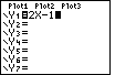
Figure 36 We enter the function on Figure 36 via the keystrokes . Figure 36 shows the screen at this point. We could use the ENTER key to mark the end of our function definition, but it is not necessary. Instead, we can press the key to move to the graph window.

Figure 37 Figure 37 has a graph of our function but it does not look like the graphs given at the top of page 128 in the text. Why? The difference comes from the WINDOW settings that we have in place. The left graph in the text is using the ZDecimal settings. We can return to the ZOOM menu to select similar settings for our graph.

Figure 38 Again, the ZOOM menu gives us a number of choices, and again we want to select ZDecimal. Therefore, press the key. This selects the option and rreturns us to the graph screen.

Figure 39 Figure 39 employs the ZDecimal settings. This graph looks identical to the left graph at the top of page 128.

Figure 40 We can verify the settings of Figure 39 by looking at the screen. We press to produce Figure 40. Here we can see that the limits for the Xmin, Xmax, Xscl, Ymin, Ymax, and Yscl are what we expect them to be.

Figure 41 We will move back to the ZOOM menu and try another option, ZStandard. The key opens the menu. ZStandard is option 6. Therefore, we press the key to select that option and to return to the graph window.

Figure 42 Figure 42 shows the graph of y=2x-1 on the ZStandard settings. This graph does not appear in the book. Rather, the right graph at the top of page 128 has the X-values going from -1 to 1 and the Y-values going from -10 to 10. We can return to the WINDOW screen to see the settings effected by the ZStandard option.

Figure 43 Figure 43 shows the settings created by the ZStandard option. We note that the Ymin and Ymax values are what we want them to be, namely, -10 and 10. However, we want to change the Xmin and Xmax values.

Figure 44 We can transform Figure 43 into Figure 44 by pressing the keys.
Having changed the settings, we press the key to return to the graph screen, shown in Figure 45.

Figure 45 Figure 45 has another graph of y=2x-1, this one with the same settings used for the graph at the top right of page 128. It is important to examine and compare Figures 37, 39, 42, and 45. All four have graphs of exactly the same function, y=2x-1. The graphs look different, but the difference arises from changes in the window settings, not from changes in the function.

Figure 32	The plot that we developed above needs to be turned off. If we were to leave it on we would keep getting the points stored in our two lists, L1 and L2, displayed on our graphs. We return to the STAT PLOT menu to turn off the plots. The keystokes to open the menus are . This produces the menu shown in Figure 32. Note that Plot1 is marked as On in Figure 32. We could go into the submenu for Plot1 and turn it off there. However, we also have option 4 on the screen, PlotsOff, which will turn off all three of the plots. We will opt for this method, and we press to select it.
Figure 33	The calcualtor responds by pasting the PlotsOff command onto the screen, shown in Figure 33. We will still need to press the key to perform the operation. After we do that, the calculator responds with the usual Done, again as shown in Figure 33.
Figure 34	Figure 34 verifies the effect of turning off all of the plots. We moved to Figure 34 by pressing the key. Note that the X-axis and the Y-axis have not changed. Our window has the same parameters that we set back in Figure 30.
Figure 35	We are now ready to enter the function y=2x-1. We do this by moving back to the Y= screen via the key. Figure 35 shows that screen and verifies that we do not have any graph functions currently defined.
Figure 36	We enter the function on Figure 36 via the keystrokes . Figure 36 shows the screen at this point. We could use the ENTER key to mark the end of our function definition, but it is not necessary. Instead, we can press the key to move to the graph window.
Figure 37	Figure 37 has a graph of our function but it does not look like the graphs given at the top of page 128 in the text. Why? The difference comes from the WINDOW settings that we have in place. The left graph in the text is using the ZDecimal settings. We can return to the ZOOM menu to select similar settings for our graph.
Figure 38	Again, the ZOOM menu gives us a number of choices, and again we want to select ZDecimal. Therefore, press the key. This selects the option and rreturns us to the graph screen.
Figure 39	Figure 39 employs the ZDecimal settings. This graph looks identical to the left graph at the top of page 128.
Figure 40	We can verify the settings of Figure 39 by looking at the screen. We press to produce Figure 40. Here we can see that the limits for the Xmin, Xmax, Xscl, Ymin, Ymax, and Yscl are what we expect them to be.
Figure 41	We will move back to the ZOOM menu and try another option, ZStandard. The key opens the menu. ZStandard is option 6. Therefore, we press the key to select that option and to return to the graph window.
Figure 42	Figure 42 shows the graph of y=2x-1 on the ZStandard settings. This graph does not appear in the book. Rather, the right graph at the top of page 128 has the X-values going from -1 to 1 and the Y-values going from -10 to 10. We can return to the WINDOW screen to see the settings effected by the ZStandard option.
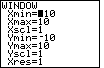
Figure 43	Figure 43 shows the settings created by the ZStandard option. We note that the Ymin and Ymax values are what we want them to be, namely, -10 and 10. However, we want to change the Xmin and Xmax values.
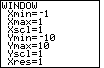
Figure 44	We can transform Figure 43 into Figure 44 by pressing the keys. Having changed the settings, we press the key to return to the graph screen, shown in Figure 45.
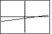
Figure 45	Figure 45 has another graph of y=2x-1, this one with the same settings used for the graph at the top right of page 128. It is important to examine and compare Figures 37, 39, 42, and 45. All four have graphs of exactly the same function, y=2x-1. The graphs look different, but the difference arises from changes in the window settings, not from changes in the function.