Central Tendency Worksheet (PC Desktop Version)
Return to Topics page
Find the mean, median, and mode values for each of the following
four sets of data.
To do this work we will employ the same strategy that we have used
in earlier examples:
- Double click on the desktop folder for our course to open it in File Explorer (Finder on a Mac)
- Now that we are in our desktop folder create a new sub-folder (sub-directory) to hold our work
- Copy our
model.R file
to that new directory
- Change the name of the model.R file to something more meaningful, ending in .R
- Start RStudio by double clickng on the new file
- Put the desired commands into the editor pane (usually by typing them into the
editor but here we will just copy and paste them)
- Save that that work in the file (you should save your work often)
- highlight the commands
that we want to run, then press the
Run icon.
- Observe the results in the Console pane
- Finally, close RStudio
Let us start the process.
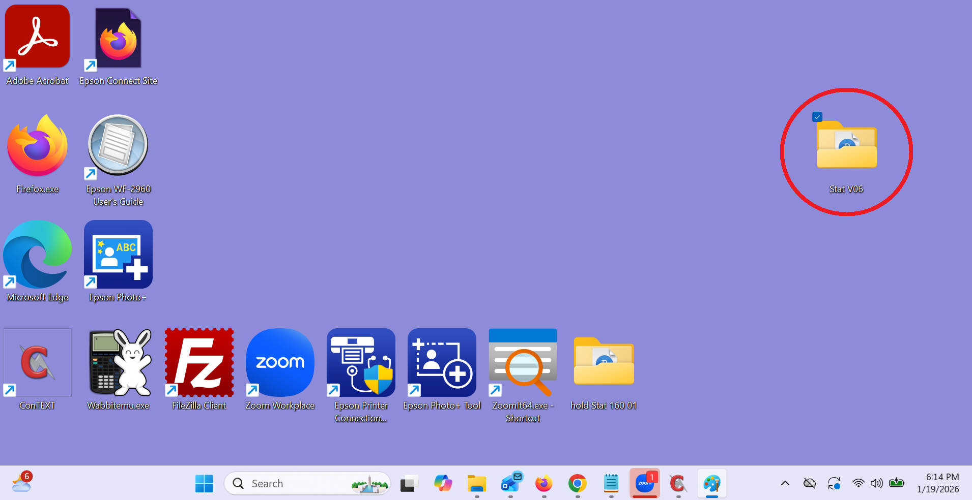
Double click on the desktop folder that we created for this course.
That folder is circled in Figure 0 below.
Figure 0
On a our Windows machine this caused the File Explorer
to open a window such as the one shown in Figure 1.
Figure 1
Click on the  icon circled in Figure 1a.
Figure 1a
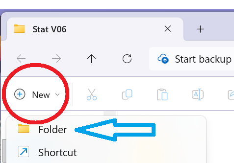
Then click on the Folder option indicated by the blue arrow in Figure 1a. This will create a
new folder, a sub-folder, here in our desktop folder. You can see the new folder in Figure 2.
Figure 2
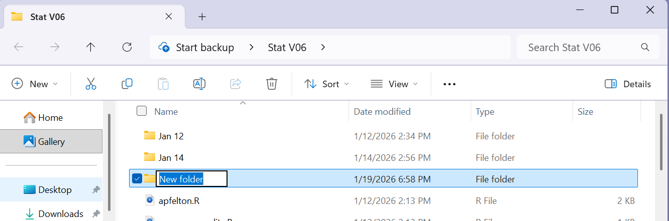
Rather than use the default folder name, New Folder
of Figure 2, type in a new name. For this project I used
 .
.
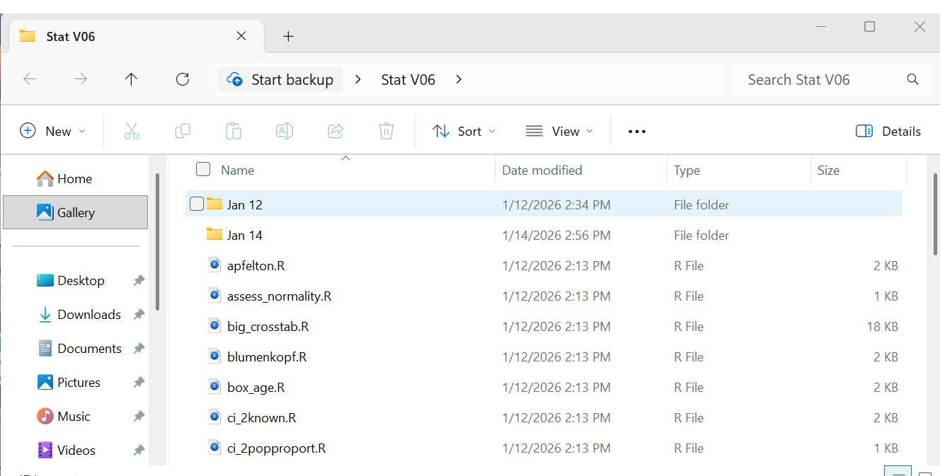
Once the sub-folder has been created and renamed, we locate the model.R
file in the list, point to it and right click to open the window
shown in Figure 3.
Figure 3
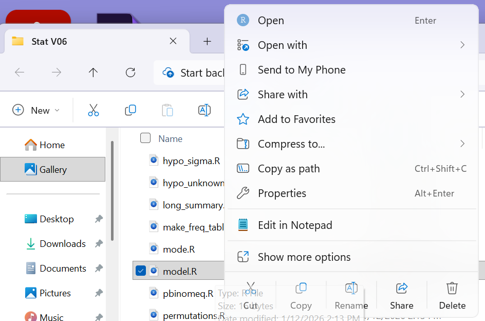
In that window we select the Copy option,
 .
.
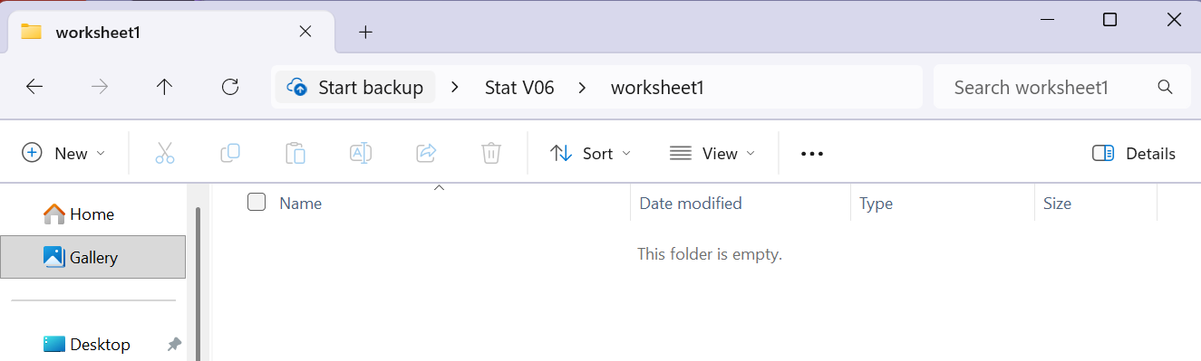
After that we return to find our worksheet1 directory and
we double click on it to open the newly
created empty directory shown in Figure 4.
Figure 4
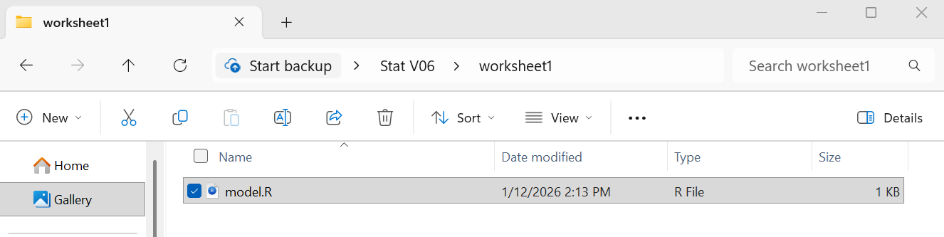
Then click on the Paste icon,
 , to paste the
 model.R
file into our worksheet1 folder. The result should look like
Figure 5.
Figure 5
We want to rename the file, in part because we do not want
to have lots of different copies of model.R
all over our various directories used in this class.
In addition, it is a good idea to have the name of the
file reflect the work you are going to do in the file.
Because the file is already highlighted, we can click on the
rename icon,  , to start the process.
This changes the display of the file, as shown in Figure 6.
, to start the process.
This changes the display of the file, as shown in Figure 6.
Figure 6
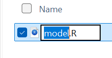
Then we can supply the new name
 .
Once that is in place we can double click on the new file name
to open RStudio, shown in Figure 7.
.
Once that is in place we can double click on the new file name
to open RStudio, shown in Figure 7.
Figure 7
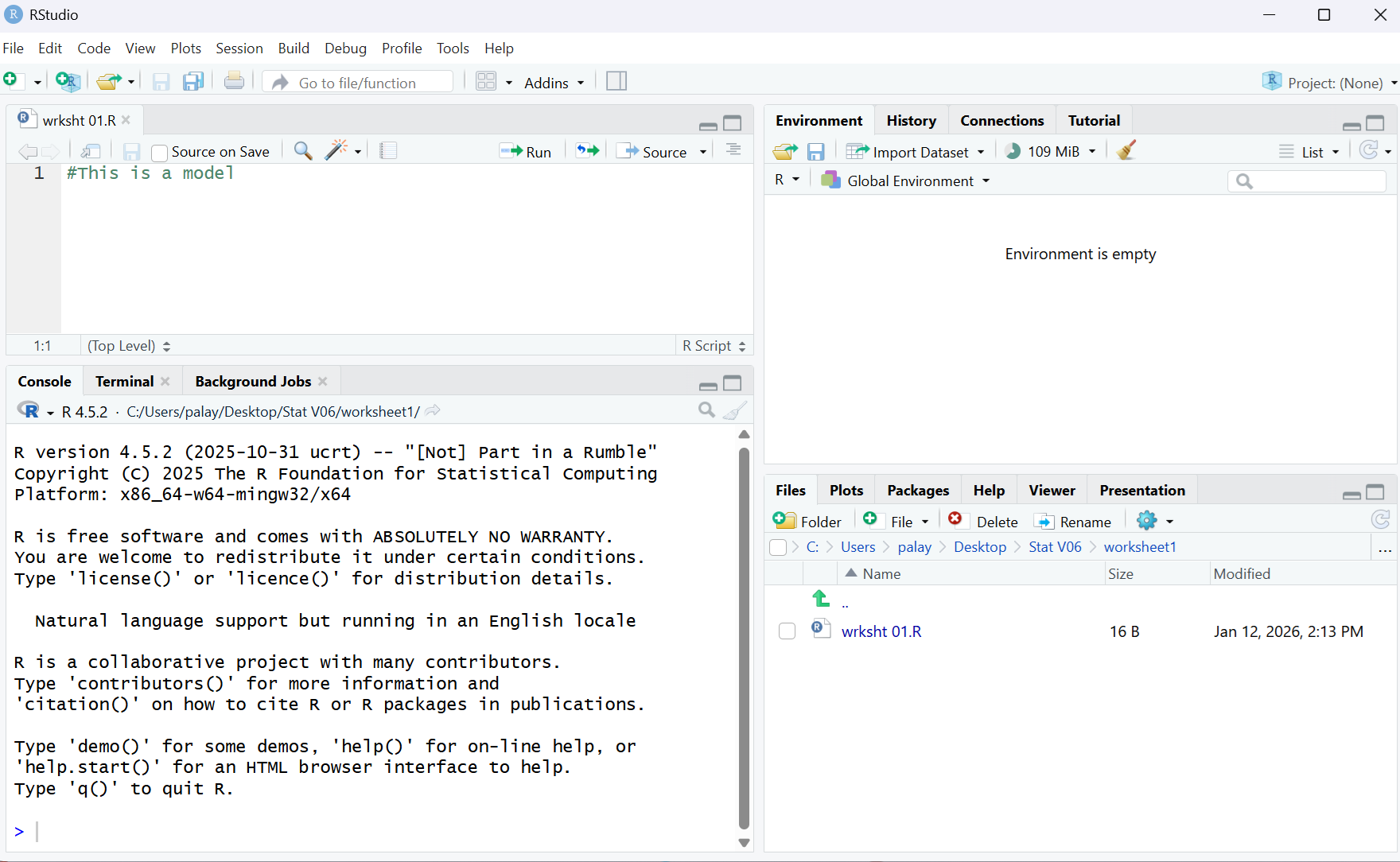
A closer examination of the Editor pane is shown in
Figure 8. This is just what we expect since
we know this to be the contents of the original wrksht 01.R
file.
Figure 8
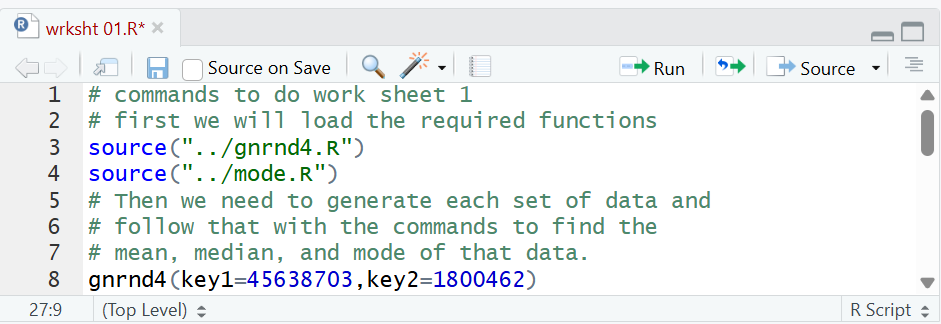
However, we want different commands.
The commands that we want are:
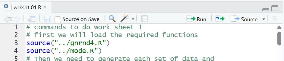
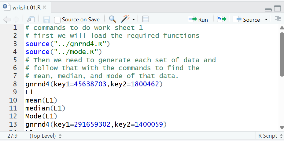
   # commands to do work sheet 1
   # first we will load the required functions
source("../gnrnd4.R")
source("../mode.R")
   # Then we need to generate each set of data and
   # follow that with the commands to find the
   # mean, median, and mode of that data.
gnrnd4(key1=45638703,key2=1800462)
L1
mean(L1)
median(L1)
Mode(L1)
gnrnd4(key1=291659302,key2=1400059)
L1
mean(L1)
median(L1)
Mode(L1)
gnrnd4(key1=604729501,key2=1100326)
L1
mean(L1)
median(L1)
Mode(L1)
gnrnd4(key1=520079004,key2=400135)
L1
mean(L1)
median(L1)
Mode(L1)
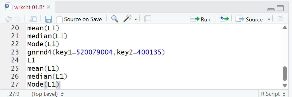
We can copy those 27 lines and paste them into the editor, replacing the
original first line.
Figure 9 shows the Editor when after we
have pasted all 27 of those lines into it.
Figure 9
Within the editor we can scroll up to see the first lines
that we added. Figure 10 shows the Editor pane
after we have scrolled to the first line.
Figure 10
We notice that the name of the file, wrksht 01.R,
shown in the file tab is displayed in
red. That is an indication that the contents
of the file have yet to be saved.
We click on the  icon to save the file.
That will change the file name to be black, as we see in Figure 11.
icon to save the file.
That will change the file name to be black, as we see in Figure 11.
Figure 11
If we turn our attention to the lower right pane in the RStudio
window, and if we click on the Files tab there,
we will see that our file is there and that it holds the
543 bytes that we put into it.
This is shown in Figure 12.
Figure 12
Now we are ready to run all of the commands that we prepared.
We could highlight and run all of the commands in the
Editor pane, but if we did so we would have to scroll through the Console
display to see all of the results. Instead, here,
we will select just the commands that we want to see at each
step of the process.
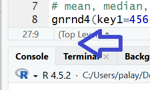
On my machine, the RStudio editor pane only shows 8 lines. I want to expand that pane.
I can point to the tiny rrectangle of area below the
editor pane, indicated by the blue arrow in Figure 12a, then left-click-and-hold
on that area and then drag the tiny arrow that shows up down to increase the size of our editor pane.
Figure 12a
In Figure 13 we see that I have increased the size of the editor pane so that it now
shows lines 1 through 13 of the file.
Figure 13
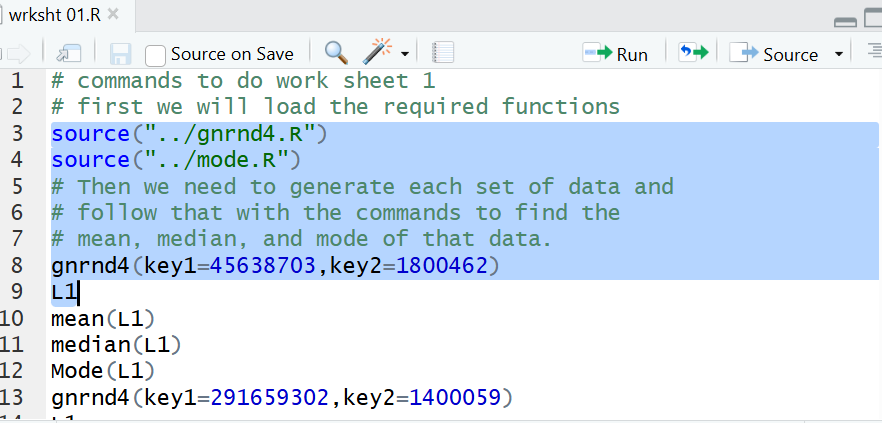
Left-click-and-hold at the start of line 3 and drag the cursor to the end of line 9.
This highlights those lines as shown in Figure 14.
Those are the commands that load our functions
and the commands to generate and view the same data that we saw above in
table 1.
Figure 14
Once that is highlighted, we click on the
 icon to have those commands performed.
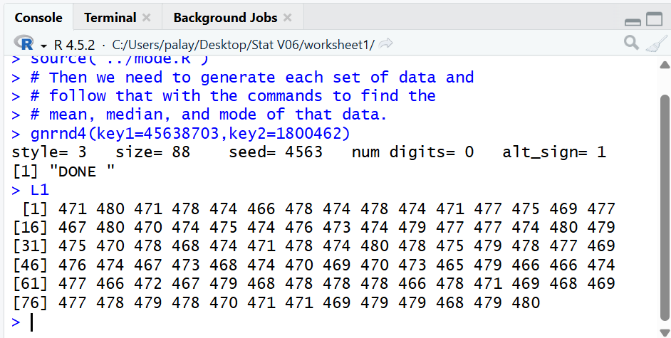
We can see the result in the Console pane, shown in Figure 15.
icon to have those commands performed.
We can see the result in the Console pane, shown in Figure 15.
We should page up on this web page to verify that
the values shown for L1 in Figure 15
are identical to the values we were given in Table 1 above.
Figure 15
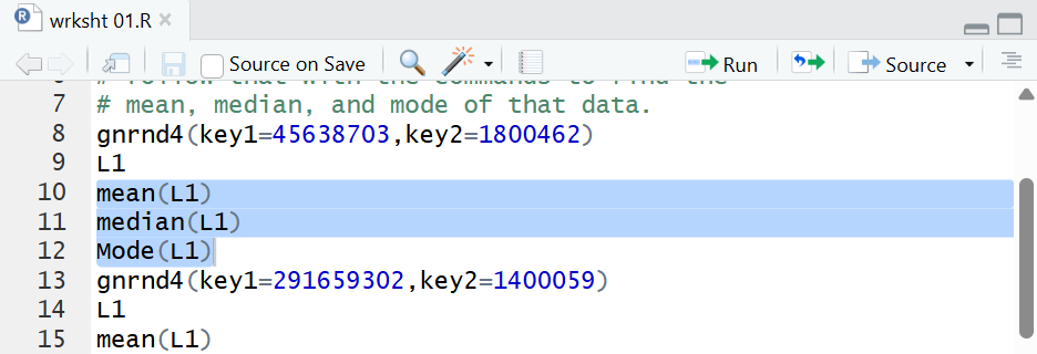
We can return to the editor page and highlight lines 10-12 as shown in Figure 15a.
Figure 15a
Clicking on the run icon, , sends
those lines to R, the result showing in
the Console pane as shown in Figue 15b.
Figure 15b
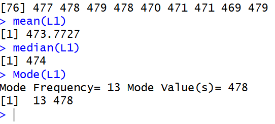
We see that the
mean is 473.7727, the median is 474,
and the mode is 478, a value that appears 13 times
in the data.
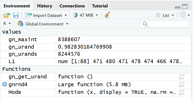
We should also note in the Environment pane, Figure 16,
that we have the variables and the functions that we expect to be defined.
Figure 16
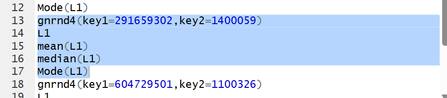
Now we are ready to work with the data in Table 2.
Therefore, we highlight the appropirate commands in the
Editor pane (lines 13 through 17), as shown in
Figure 17.
Figure 17
Then press the
icon.
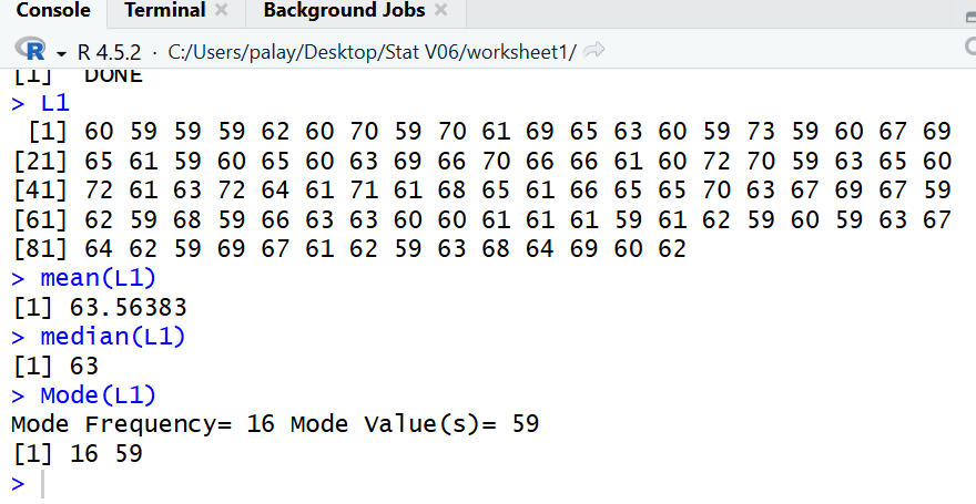
Figure 18 shows the results of those commands.
Again we verify that the values displayed are identical to those in Table 2.
And we find that the
mean is 63.56383, the median is 63,
and the mode is 59, a value that appears 16 times
in the data.
Figure 18
Returning to the Editor pane we highlight
the next set of commands in lines 18-22.
Figure 19
Then we run them to get Figure 20.
Figure 20
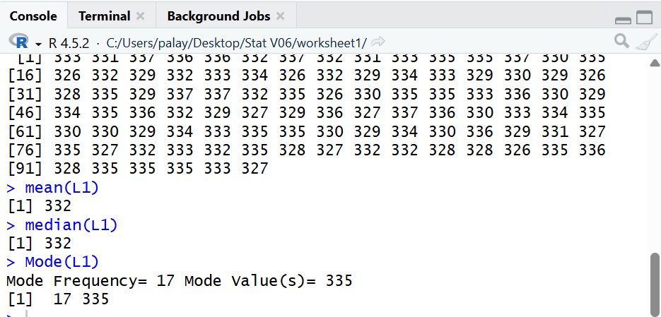
Again we verify that the values displayed are identical to those in Table 3.
And we find that the
mean is 332, the median is 332,
and the mode is 335, a value that appears 17 times
in the data.
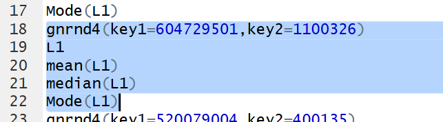
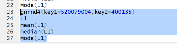
That leaves just the last set of commands to highlight, as shown in
Figure 21.
Figure 21
Then we run them to get Figure 22.
Figure 22
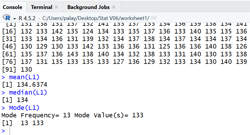
Again we verify that the values displayed are identical to those in Table 4.
And we find that the
mean is 134.6374, the median is 134,
and the mode is 133, a value that appears 13 times
in the data.
We have found all the values we needed to find.
Therefore, we can quit R using any of the different
exit points, the easiest being the upper right corner
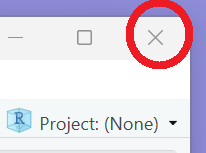 .
This will pop up a window,
shown in Figure 23, to ask if we want to save the environment.
.
This will pop up a window,
shown in Figure 23, to ask if we want to save the environment.
Figure 23
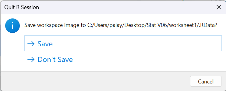
We can click on  to do this.
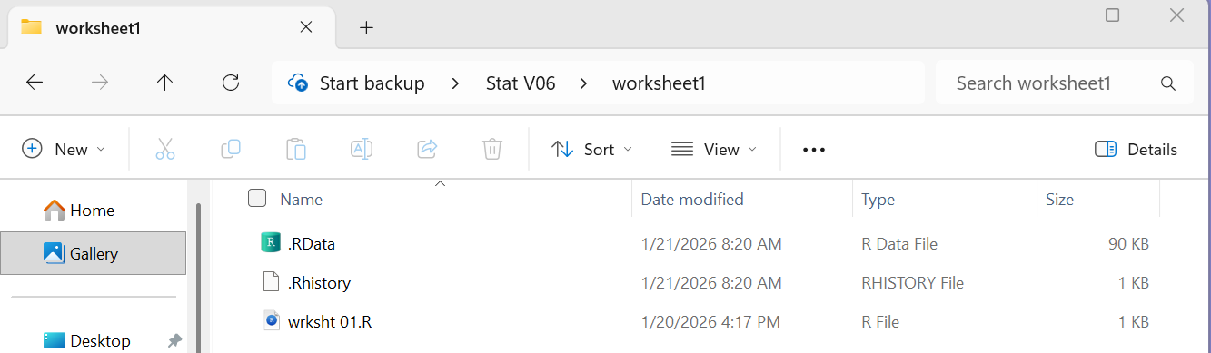
Once we have left RStudio, we can see, in
Figure 24, the File Explorer shows
that we have three files in our directory.
Figure 24
Return to Topics page
©Roger M. Palay
Saline, MI 48176 January, 2026