Stem and Leaf Plot

Return to Topics page
Stem and Leaf Plots were quite helpful, in some cases, when we had to organize data by hand. The concept is best illustrated. Consider the data in Table 1 A quick read of the data, just looking for the lowest and highest values suggests that the range of values is from the 320's to the 370's. We create a list of stems from 32 to 37 as

32:
33:
34:
35:
36:
37:

Then, we read the values in the table, one at a time, and for each value we find the stem that has the first two digits of the value. So for 371 we locate stem 37:. We write the units digit of the value, in the case of 371 that would be 1, after the stem. Now our diagram becomes

32:
33:
34:
35:
36:
37:1

We move to the next item in the table, 354. For that value we append the units digit 4 to the stem 35:. The diagram is now

32:
33:
34:
35:4
36:
37:1

We move to the next item in the table, 352. For that value we append the units digit 2 to the stem 35:. We already had 35:4 there so that becomes 35:4 2. The diagram is now

32:
33:
34:
35:4 2
36:
37:1

We keep building the diagram, appending the units digit 4 from 344 to the 34: stem, appending the units digit 7 from 337 to the 33: stem, and appending the units digit 4 from 354 to the 35: stem which now becomes 35:4 2 4 and the diagram becomes

32:
33:7
34:4
35:4 2 4
36:
37:1

This simple methodical process, when finished, produces the diagram

32: 3 9 8 7 7
33: 7 9 4 9 8 6 1 9 7 8 7 3 8
34: 4 5 3 6 3 8 4 1 3 1 2 8 8 7 4 9
35: 4 2 4 9 0 4 9 0 2 2 2 9 0 7 8 4 2
36: 8 0 7 3
37: 1

That result is an "unsorted" stem and leaf diagram. It gives us a feeling for the distribution of the data. In fact, it really gives us a "sideways" histogram of the data with intervals [320,329), [330,339), [340,349), [350,359), [360,369), and [370,379). Figure 1 shows the usual histogram produced by the statements

gnrnd4( key1=121855504, key2=0001000345 )
hist( L1, xlim=c(320,380), breaks=seq(320,380,10),
      ylim=c(0,20), yaxp=c(0,20,20), las=1,
      cex.axis=0.6, right=FALSE)

Figure 1

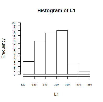
The stem and leaf diagram from above has the same number of bars, 6, and the length of the stem and leaf bars, the number of units digits in each bar, is the height of the corresponding bar in Figure 1.

The additional feature of the stem and leaf diagram is that we could actually move back from the diagram to the original data. thus the line 32: 3 9 8 7 7 represents the values <323, 329, 328, 327, and 327.

Having organized the information from Table 1 into the stem and leaf diagram, we could sort the data by just sorting the units digits, the leaf values in each line. This would produce

The shape remains the same, thus giving us the simple histogram shape, but, with the values in order we also see more details of the distribution of the values. We could even use this "sorted" stem and leaf diagram to help identify the median and quartile points. Even the mode becomes more obvious in this sorted version, the five 2's in the 350's just stand out as being the most frequent values.

Of course, all of this, while cute, is still a pain once we have a computer to do our work for us. In addition, the stem and leaf process, as shown above, just works for situations where the stem ends at the ten's digit and the leaf is just the unit's digit.

What would we do for the data in Table 2? These values range from 2096 to 2549. If we were to follow the pattern introduced above we would end up with stem values from 209 to 254, that is, we would have 46 stem values. We can pretty much assume that some of these would have no leaves, some would have 1 leaf, some would have 2 leaves and there may even be some with 3 or more leaves. We have room on this web page to display such a diagram, although we will omit the stems that have no leaves.

This gives us some information, though it is distorted by the missing lines.

Traditionally, in such a situation, we would recognize that we would get a better feel for the distribution of the values in Table 2 if we had the stems end at the hundred's digit and the leaf would be the ten's digit. Doing this would mean that we would be losing some information, namely the unit's digit, but we would end up with fewer stems, in this case we would have stems 20, 21, 22, 23, 24 and 25. Rather than just using the data as it is and lopping off the unit's digit, we would actually round the values of Table 2 to the nearest ten's digit to get the values in Table 3. From there we can just divide those values by ten to get Table 4. Now we can use the original process to produce the following:

Then we could sort that to get

Of course, when reading this we need to remember how we got the values and that 21: 0 2 7 8 9 9 represents 6 values from the range of 2195 to 2295 because we rounded the values to the ten's place and then divided them by 10 to shift the values so that we could use our stem and leaf procedure. text to be added

It should be evident that the stem and leaf procedure was quite helpful before we had computers but that it does not serve much more than a historical use now. R does have a built-in function stem() that will produce a ste and leaf diagram. if we run stem(L1) for the current data get the output shown in Figure 2.

Figure 2

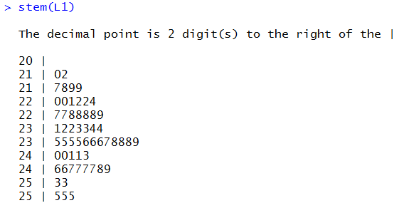
You should note that R has taken the liberty of dividing the intervals in half. That way we get two entries for the stem 21, the first holding any leaf values from 0 through 4 and the second holding leaf values from 5 through 9. This makes the branches shorter. Also, note that the stem() function took it upon itself to decide where to locate the break between the stem and the leaf.

As noted above, we have little need for these diagrams at this point. Still, it is nice that R has a built-in function to do our work if we need to produce such a diagram. We could also create our own function, perhaps with a bit more flexibility. For example, the function definition

stem_leaf<-function(
  lcl_list, place=0)
{ # convert the list to the form dddsl where the l is
  # the leaf and the s becomes the stem
  chop_list <- floor(round( lcl_list, -place)/(10^place))
  # we can sort this 
  chop_list <- sort( chop_list )
  # then produce the stems and the leaves
  leaf_list <- chop_list %% 10
  stem_list <-floor( chop_list/10)
  n <- length(stem_list)
  branch <- paste(stem_list[1]," | ",leaf_list[1],sep="")
  old_stem <- stem_list[1]
  for (i in 2:n)
  {
    if( stem_list[i] == old_stem)
    { branch <- paste( branch, leaf_list[i], sep=" ")}
    else
    { cat( branch, "\n")
      branch  <- paste(stem_list[i]," | ",leaf_list[i],sep="")
      old_stem <- stem_list[i]}
  }
  cat( branch, "\n" )
}

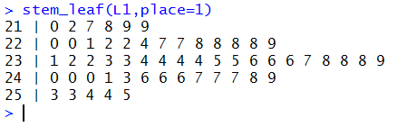
really does the exact process that was described above. That function is available at stem_leaf.R. For that function you supply not only the list of data values but also the place where you want the leaf. So, if we want to have the leaf in the ten's place, we give the command stem_leaf(L1,place=1) and R will produce the output shown in Figure 3.

Figure 3