Probability: Normal Distribution
Return to Topics page
Introduction
The normal distribution is defined by a mathematical formula,
namely,
 where we are given values for the mean, μ,
and the standard deviation, σ.
With such a definition we get a different value
for each different combination of μ and σ.
Fortunately, we can look at a single example, called the standard normal distribution,
where we have μ=0 and σ=1.
With those values the general formula becomes
where we are given values for the mean, μ,
and the standard deviation, σ.
With such a definition we get a different value
for each different combination of μ and σ.
Fortunately, we can look at a single example, called the standard normal distribution,
where we have μ=0 and σ=1.
With those values the general formula becomes
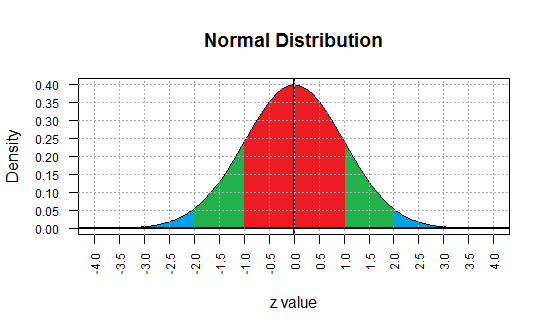
 A graph of that function appears in Figure 1.
Remember that as a probability density function, the area under the curve
and above the axis is equal to 1 square unit. Each small rectangle in Figure 1 represents
0.5*0.05 or 0.025 square units. It takes 40 such areas to equal 1 square unit.
A graph of that function appears in Figure 1.
Remember that as a probability density function, the area under the curve
and above the axis is equal to 1 square unit. Each small rectangle in Figure 1 represents
0.5*0.05 or 0.025 square units. It takes 40 such areas to equal 1 square unit.
Figure 1
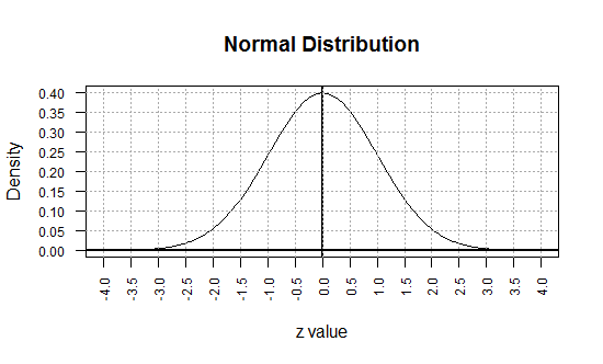
We must note here that the curve never gets to the x-axis. That is, the curve is
always above the x-axis even for values more extreme than -4 or 4.
The normal distribution is often called a bell-shaped curve
for the obvious reason that the graph of the function can be
made to look somewhat like a bell.
A careful "read" of the graph in Figure 1 reveals that we are calling values along the traditional
x-axis z values. This is not a typo. It is quite important.
We refer to the values along the traditional x-axis as z values;
we will learn, later, how to change values from a non-standard normal distribution
into z values.
The "can be made to look somewhat like" is added
to point out that part of the visual effect of the curve depends upon
not having equal x and y scales.
In Figure 1 we go from -4 to 4 on the x scale, but
we magnify the y scale by stretching it so that the vertical spread
shows 0 to 0.40.
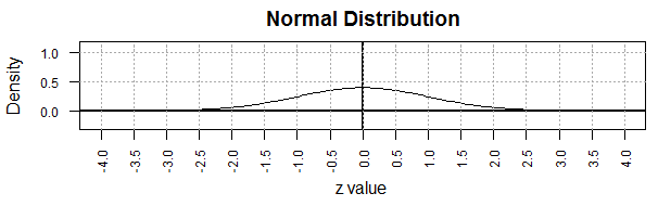
If we had equal scales the curve would appear
as in Figure 1a. This figure is no more or less accurate in
displaying the normal curve, but Figure 1a
no longer gives that impression of a "bell" shape.
Figure 1a
Looking back at Figure 1 (or at Figure 1a if you like)
we see that the
normal distribution is a symmetric distribution.
Since the probability that a random variable,
X, is less than a given
z value is the area under the
curve and to the left of the vertical line at that value,
this symmetry means that P(X<0)=0.5.
Because the standard normal distribution has mean zero, μ=0,
and standard deviation one, σ=1,
the region of the graph between -1 and 1
on the graph represents values that are within 1 standard deviation of the mean.
The area under the curve between -1 and 1
is about 0.68.
(A better value would be 0.68269, but we will just use 0.68 for now.)
Therefore, again using symmetry, the red area in Figure 2
represents two pieces, each accounting for about 34% of the total area.
Figure 2
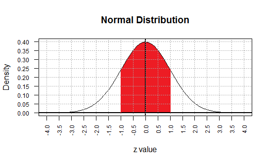
Knowing the values shown in Figure 2 we can say that
P(X < -1) ≈ 0.16, or
P(X > 1) ≈ 0.16, or
P(X < 1) ≈ 0.84, or
P(X < -1 or X > 1) ≈ 0.32.
Quite a bit of knowledge from just one graph!
If we move out another standard deviation, we find that the region between
-2 and 2 accounts for about 95% of the total area (1 square unit)
under the curve.
(A better value would be 0.954499876, but we will just use 0.95 for now.)
Figure 3
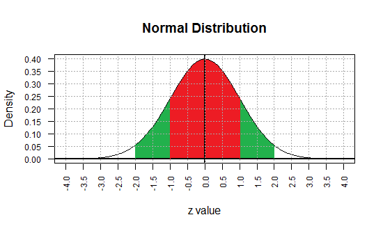
Using symmetry and the earlier information we have assigned probabilities to the various regions in
Figure 3. Now we can say that
P(X < -2) ≈ 0.025, or
P(X < 2) ≈ 0.975, or
P(-2 < X < 1) ≈ 0.815,
and so on.
Extending our range, the area under the curve between -3
and 3 is about 0.997 square units.
Figure 4
Thus, 99.7% of all the area under the curve is
within 3 standard deviations of the mean.
The Table
As we have seen in the general discussion of continuous probability functions,
having these graphs is nice, but having a table would be even nicer.
We do have access to a
Normal Distribution Table.
In addition, there is a different web page that is meant to
help you with Reading Tables.
As noted on that page, there are many different styles of
tables in general use for the normal distribution.
If you have a powerful calculator or a computer, it is much less likely that
you will need to use tables.
However, reading such tables is not a bad skill to acquire.
There are just four kinds of probabilities that we want to
evaluate for z values in a standard normal distribution.
They are
- P(X < z)
- P(X > z)
- P(z1 < X < z2)
- P(X < z1 or X > z2)
Approaches to solving all of these were presented on the
Probability: Continuous Cases web page.
Here we will just run through an example of each, but
with minimal discussion.
An example of the first problem might be to find P(X < -2.14).
Figure 5 displays the portion of the table,
from the Normal Distribution Table,
that we need for this.
Figure 5
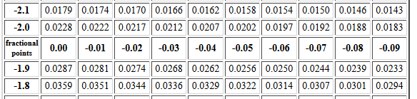
Having looked at the web page that holds this table,
we know that this table
gives the area under the curve to the left of the z value.
Therefore, we can just read the correct answer as 0.0162.
An example of the second problem
might be to find P(X > 0.97).
Figure 6 displays the portion of the same table
that we need for this.
Figure 6

In this case we want to use the fact that
P(X > 0.97) = 1 - P(X < 0.97).
Therefore, our answer will be 1 - 0.8340 = 0.1660.
An example of the third style of problem might be to find
P(-2.14 < X < 0.97).
We know that this will be equal to
P(X < 0.97) - P(X < -2.14).
Reading the required values from the table gives this as
0.8340 - 0.0162 = 0.8178.
Using the same z values, an example of the fourth style might be
to find
P(X < -2.14 or X > 0.97).
We could approach this as just finding the sum
P(X < -2.14) + P(X > 0.97)
which is 0.0162 + 0.1660 = 0.1822.
Alternatively we could compute this as
1 - P(-2.14 < X < 0.97),
or 1 - 0.8178 = 0.1822.
pnorm() in R
Of course, our goal is to see how we can do all of this
in R. The design and use of the functions papfelton()
and pblumenkopf was presented on the
Probability: Continuous Cases web page.
Those functions were modeled upon the R function
pnorm(), a function that, in its most simple form, will give
the area under the standard normal distribution curve
and left of a specified z value.
Thus, we can find
P(X < -2.14)
by using the command pnorm(-2.14), and we can find
P(X > 0.97)
by using the command 1 - pnorm(0.97).
These are shown in Figure 7.
Figure 7
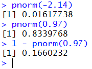
These are the same results we found above using the table,
although these have more significant digits.
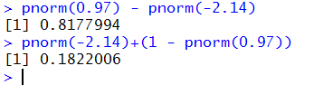
We can find
P(-2.14 < X < 0.97) by finding
P(X < 0.97) - P(X < -2.14)
which we write as pnorm(0.97) - pnorm(-2.14).
We can find
P(X < -2.14 or X > 0.97)
by finding
P(X < -2.14) + P(X > 0.97)
which we rewrite as
P(X < -2.14) + (1 - P(X < 0.97))
which we then code as pnorm(-2.14)+(1 - pnorm(0.97)).
These are shown in Figure 8.
Figure 8
When we use pnorm() we may specify an argument
that changes its behavior from
the default of finding
the area under the curve to the left of the z value to
finding the area under the curve to the right of the z value.
The former is called the left tail or lower tail area.
The latter is called the right tail or upper tail area.
The new argument for pnorm() has the name lower.tail
and, if given, it must be assigned the value TRUE or FALSE.
By default, it is understood to be TRUE
and, as a result, pnorm() by default produces the
lower tail area.
If, however, we specify lower.tail=FALSE
then the function produces the upper tail area.
We have already seen that we can get the
upper tail area by subtracting the lower tail area from 1.
That is how we found P(X > 0.97).
We calculated 1 - P(X < 0.97).
Using the parameter lower.tail=FALSE we can get the same value
directly from pnorm(0.97,lower.tail=FALSE) as shown at
the start of Figure 9.
Figure 9

Figure 9 also shows an alternative to coding our fourth example above.
The use of the lower.tail=FALSE argument saved us from having to construct
the expression (1 - some left-tail probability).
We get the same answer either way.
Both are correct. Use the form that best suits you.
Reading "backward" from the table
In our earlier discussion of general continuous probability functions
our next step was to read the table backwards.
That is, we want to find a z value such that
P(X <z)=0.05.
We learned how we could find bracketing values in the table and
then interpolate between them to find a good approximation to
the desired z value.
Figure 10 shows the portion of the table that we want to use for
this problem. The two bracketing cells are highlighted.
Figure 10

The z values associated with those two cells
are -1.64 and -1.65. We want to be halfway
between the two cell values, 0.0505 and 0.0495.
Therefore, our approximation will be halfway between the
two z values, (-1.64 +-1.65)/2 = -1.645.
qnorm() in R
The R function that does this "backwards" work is
qnorm(). In R we could get the answer to
finding a z value such that
P(X <z)=0.05
by using the command qnorm(0.05) as is shown in Figure 11.
Figure 11
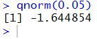
Again, we get a better answer from R than
we could get from the table
because the table values are all rounded to 4 decimal places.
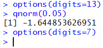
As we have seen in other pages, even the value shown
in Figure 11 is a rounded value.
We could get R to give us more digits in the answer, as shown in
Figure 12, but there is really no need to do this. For our work there is
really no need to go beyond four significant digits (the table result).
Figure 12
The work above used the standard normal distribution,
the distribution that has mean zero (μ = 0)
and standard deviation one (σ = 1).
That is an ideal distribution. We have a table for P(x < z)
for that distribution. We have the functions
pnorm() and qnorm() for that distribution.
But what do we do when we have a non-standard normal distribution?
That is the BIG QUESTION.
The next section leads us to the
BIG ANSWER.
Normalizing a non-standard normal distribution
Here is a separate script
that can be used to demonstrate the same concepts shown
below. To use the script download it to an appropriate directory
or open it and then copy it to an appropriate script file.
Or, istead of using the script,
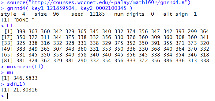
consider the data in Table 1.
Figure 13 shows the generation of that same data along with
a computation of the mean and, seemingly, the standard deviation.
Figure 13
Although it is tempting to just move ahead at
this point, we will pause long enough to
remember that sd() computes the standard
deviation of a sample.
For this discussion we want to use the standard deviation of a population.
Recall in the much earlier discussion of computing standard deviations
we developed a small function, pop_sd() to compute the
standard deviation of a population.
The code for that function was
pop_sd<-function( input_list )
{ n <- length( input_list)
sd( input_list )*sqrt((n-1)/n)
}
Figure 14 shows this function entered into R
along with a new computation for the value of σ.
Figure 14

At this point we have assigned the mean to a variable called mu
and we know that mu holds the value 346.5833, and the
standard deviation, 21.19191 is stored in sigma.
Before we go further it might be worth looking at
the distribution of values in L1.
We start by looking at a summary(L1) just so that we can find
the minimum and maximum values, and then move to a histogram command.
(It is a bit disingenuous to throw out this rather long histogram command
as if I just created it by looking at the values from the summary.
The truth is that I slowly developed the command, adding directions along
the way, changing those directions as I reviewed the resulting graph.
The command that you find here is the result of that development.)
Figure 15

The graph produced is in Figure 16.
Figure 16

The distribution shown in Figure 16 is
clearly not that shown in Figure 1.
But that is not a surprise.
Figure 1 shows an "ideal" distribution defined by a mathematics.
Figure 16 shows a real population with just 96 values in it.
Still, the distribution of L1 shown in Figure 16 is at least
"approximately" normal.
(It is also good to remember from our earlier presentation
on histograms that the decision that we made on the number of intervals
and the placement of the intervals does influence the
appearance of that histogram.)
We know, from Figure 13, that we have stored the mean in the
variable mu. We will create a new population by
subtracting the mean from each value in L1. The statement
L2 <- L1 - mu does just that.
If we follow that with the statement L2
we get to see all 96 of the values in the new variable L2.
This is shown in Figure 17.
Figure 17

We did not have to look at all those values, but such a listing provides
a nice confirmation of the action that we have taken.
Now we can look at the new population
in L2. Figure 18 shows the commands and the results
for finding the mean, population standard deviation and
the Min and Max values of L2.
Figure 18 ends with a new hist() statement to display
the distribution of the new population.
Figure 18
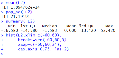
Please note that 1.894762e-14
means 1.894762*10-14
which we could expand to 0.00000000000001894762,
a value that is essentially zero.
When that value is rounded to 3 decimal places by the summary(L2)
command it is displayed as 0.000.
Another point to note is that the standard deviation of L2
is exactly the same as the standard deviation of L1.
This is an important fact:
Adding the same value (or subtracting the same value)
from every element in a population produces a new population but this new
population will have the same
standard deviation as did the original population.
We could even use our R function to express this.
If k is any particular single value,
then for a population Ln it will always be true that
pop_sd(Ln) == pop_sd(Ln + k)
where we understand == to mean is equal to.
This should make sense because the standard deviation is a measure of
dispersion. It is a measure of the deviations from the mean.
All we accomplished by subtracting the mean
from every element of L1 was to shift all the values
from being centered around
approximately 346.5833 to being centered around approximately 0.00.
We did not alter the deviations of the values from the mean value.
The shape of the distribution in Figure 18 is like
the shape of the distribution in Figure 16.
Again, changing the intervals
would alter the appearance of the graph, but not by all that much.
The graph would still
generally resemble that of a normal distribution.
Figure 19

Now take the values in L2 and divide each of them by sigma,
the standard deviation of L1, which we know is also the
standard deviation of L2. Put the results in the variable L3
and then display L3. This is shown in Figure 20.
Figure 20
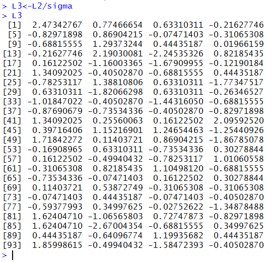
Now that we have a new population we will examine
its values as shown in Figure 21.
Figure 21

The mean of L3 is even closer to 0,
as we would expect since we divided
each value in L2 by a number around 21.19191.
The standard deviation of L3 is essentially 1.0,
where we need to say "essentially" because
all we can see is that R has rounded the value to
1. This is another important observation:
Multiplying (or dividing) every element in a
population by the same value
produces a new population but this new
population will have a new standard deviation
that is equal to the standard deviation of the
original population multiplied (or divided) by that same value.
We could even use our R function to express this.
If k is any particular single value
then for a population Ln it will always be true that
pop_sd(Ln * k) == k * pop_sd(Ln)
where we understand == to mean is equal to.
Figure 21 ends with a new hist() statement to display
the distribution of the new population. That histogram appears in Figure 22.
Figure 22
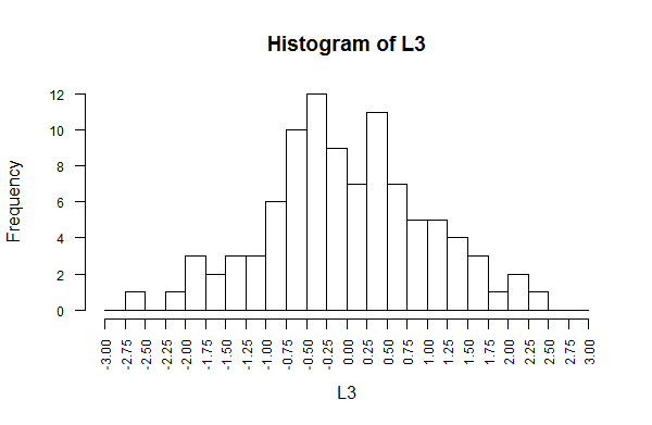
Again, this resembles the shape of Figure 1.
In addition, this new population, L3, has mean=0
and standard deviation=1.
If we have a population Lorig
that has mean=μ and
standard deviation=σ then we can get a new population
Lnew by subtracting μ from each
value in Lorig and
then dividing that difference by
σ. When we do this the
new population Lnew will have mean=0
and standard deviation=1.
Here is a link to a script demonstrating this.
The Big Answer: z-scores
If x is a value in Lorig then
using that transformation produces a new value, we will call it z
in Lnew
where  Furthermore, z will have mean=0 and standard deviation=1.
This is the BIG ANSWER for the question above:
How do we deal with a normal
distribution that has a mean different from 0 and/or
a standard deviation different from 1?
The answer is that we use this z = (x - μ) / σ
to convert any value in this non-standard population to a z-score
and then we can use our table
or our pnorm() function to answer questions about that value.
Furthermore, z will have mean=0 and standard deviation=1.
This is the BIG ANSWER for the question above:
How do we deal with a normal
distribution that has a mean different from 0 and/or
a standard deviation different from 1?
The answer is that we use this z = (x - μ) / σ
to convert any value in this non-standard population to a z-score
and then we can use our table
or our pnorm() function to answer questions about that value.
For example, IQ scores have a normal distribution with mean equal to 100 and
standard deviation equal to 15.
If this is the case then what is P(X ≤ 88)?
We find the z-score equivalent to 88
by doing the computation (88-100)/15=-12/15≈-0.8.
Then, if we are using the table, we look up that z-score in the table.
Figure 23 shows that part of the table.
Figure 23
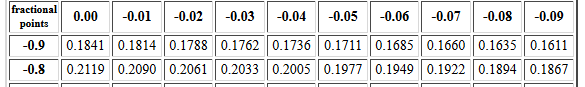
From the table we see that P(z≤-0.8)=0.2119,
therefore P(X≤88)=0.2119.
Alternatively, we could just use the pnorm(-0.8) command
and let R do the work. Figure 24 shows exactly that
approach.
Figure 24
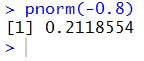
In Figure 24 we see the slightly more accurate answer.
|
This is a great time to point out just how sloppy we have gotten.
We talk about IQ scores as being normally distributed with mean 100 and standard deviation of 15.
Yet, if we think about it, this is absurdly wrong.
IQ scores are whole numbers. You do not get an IQ score of 104.24!
IQ scores are not continuous. Normal distributions are continuous.
It is impossible to have discrete distributions be normal distributions.
And yet, we refer to IQ scores as a normally distribution.
We will return to this complication in the box below
the following examples, after the answers following Figure 25.
|
We use the same approach to answer questions such as
- Selecting a random person, how strange is it for that person to have an
IQ greater than or equal to 138?
- What portion of the population has an IQ between 85 and 105, inclusive?
- What is the likelihood of selecting a
random person whose IQ is outside the range
from 94 to 119?
Those questions become
- P(X ≥ 138)
- P(85 ≤ X ≤ 105)
- P( X < 94 or X > 119 )
We convert the values in these problems to z-scores
- 138 becomes z=(138-100)/15=38/15≈2.53333
- 85 becomes (85-100)/15=-15/15 = -1.000
105 becomes (105-100)/15 = 5/15 = 0.33333
- 94 becomes (94-100)/15 = -6/15 =-0.4
119 becomes (119-100)/15 = 19/15 ≈ 1.26666
Then we can transform the original problems into
problems using those z-scores.
- P(X ≥ 138) = P(z ≥ 2.5333) = 1 - P(z ≤ 2.5333)
- P(85 ≤ X ≤ 105) = P(-1 ≤ z ≤ 0.3333) = P( z &le:0.3333) - P( z ≤ -1 )
- P( X < 94 or X > 119 ) = P( z < -0.4 or z > 1.2666) = 1 - (P(z < 1.2666) - P(z < -0.4) )
If we are using the table then we need to look up all these values
in the table. A value of 2.5333 poses a problem in that the table
gives us values for 2.53, namely 0.9943, and 2.54, namely
0.9945, but that is as close as the table comes. Since we want the value that is
1/3 the way between 2.53 and 2.54,
and since the change in the probability is
0.9945-0.9943=0.0002, we can interpolate a value that is 0.0002/3
beyond 0.9943 or 0.9943+0.0000666≈0.99437.
You see why using the tables is a pain!
Rather than get bogged down with the tables, we could just get the answers using R.
The problems restated in R become
- 1-pnorm(2.5333) or pnorm(2.5333,lower.tail=FALSE)
- pnorm(0.3333)-pnorm(-1)
- 1-(pnorm(1.2666)-pnorm(-0.4) )
Figure 25 shows all of these:
Figure 25

Reading the answers from Figure 25 we get
- P(X ≥ 138) ≈ 0.00564971
- P(85 ≤ X ≤ 105) ≈ 0.4718908
- P( X < 94 or X > 119 ) ≈ 0.4472274
Here we return to the question of calling the IQ distribution,
which we know to be a discrete distribution, a normal
distribution. We do this because the distribution of the IQ scores
approximates a normal distribution. It is just easier for us the
deal with the distribution as a normal one rather than as a discrete one.
However, we should recall that in a continuous
distribution the probability of getting an
exact value is zero (remember that there is a height of the curve in Figure 1
above every point, but there is no width at a point and area is length times width
which means the probability is zero).
A consequence of this is that when we find, as we did above,
P(X≥138) we really are not sure just what that means
because there really should be a P(X=138). If we want to include 138
and all the values above it, then
we should really have looked at P(X>137.5).
Using the halfway point between our discrete IQ values
makes a lot of sense. We would say, then,
that P(X=138) = P(137.5<X<138.5).
At this point we would have to translate those values to z-scores, but in R
we could let the system do this by expressing that as
pnorm((138.5-100)/15)-pnorm((137.5-100)/15).
The console view of this is:
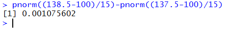 We say that P(X=138) = P(137.5<X<138.5) = 0.001075602.
The little trick of having R compute the z-scores as we just did
could have been used in the earlier computations. Of course, now we know that we should
have done all of those using the halfway points.
Here are the corrected statements, done without finding the
z-scores ourselves.
 You can see that the answers change, but not by much.
|
As you have seen, z-scores and the relation
have been essential
for converting values from non-standard normal distributions to our
standard normal distribution.
In the same way, solving the relation for x
to get x = z*σ + μ,
we can go backwards from the standard normal distribution to
a non-standard one.
For example, for a distribution that is normal with mean 75 and standard deviation 14,
we want to know the value in that distribution that has 12%
of the values less than it.
In a standard normal distribution
we would find the z-score by looking up the area in
a cell of the table, or by using the qnrom(.12) function.
Figure 26 shows the portion of the table that we could use.
Figure 26
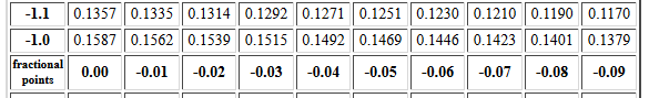
The two cells that bracket 0.12 hold 0.1210 and 0.1190,
and they hold the values
for -1.17 and -1.18, respectively.
We need to be halfway between so our table generated z-score
will be -1.175.
The R command is shown in Figure 27.
Figure 27

Here we get a z-score of -1.174987.
The R-generated value is almost identical,
so we will just use -1.175
as the z-score.
Then, using x = z*σ + μ,
we can find the value
in the non-standard distribution by calculating
-1.175*14+75 = -16.45+75 = 58.55.
Of course, using the R value we could have done this as
qnorm(.12)*14+75 as is shown in Figure 28.
Figure 28
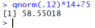
All done in one step!
The N(μ,σ) Notation
Let us take a minute here to introduce a shorthand method for
saying that a distribution is normal
with mean=a and standard deviation=b.
That shorthand is to say that the distribution is N(a,b).
The standard normal distribution is N(0,1).
We say that a normal distribution with
mean 75 and standard deviation 14 is N(75,14).
The Expanded Notation for pnorm() and qnorm()
It should not come as a surprise that most of our real
work will be with non-standard normal distributions.
If you understand that for ages we have had but the one table of the
Standard Normal Distribution, then you must appreciate the
importance of the z-scores, the relation
, and the relation
x = z*σ + μ.
Furthermore, unlike the discrete binomial distribution,
you must appreciate that it would be
impossible to produce tables for all of the different combinations
of non-standard values for the mean and standard deviation
of these non-standard normal distributions.
However, our calculators and computers do not rely
on tables to do their work. Therefore, it is possible for
our technology to deal directly with non-standard situations
as long as we supply the non-standard values for the mean and standard deviation.
In particular, in R the pnorm() function
actually allows us to specify one or both of those values.
For a distribution that is N(75,14), to find the
P(X < 83.4) we just need to
give the command pnorm(83.4, mean=75, sd=14) as is shown in
Figure 29. Of course, we could do the extra work the way
have done it above, also shown in Figure 29, but using the arguments
seems a bit cleaner and easier to understand.
We get the same answer either way.
Figure 29

The four answers, and then corrected answers,
to the three example problems from earlier (see Figure 25
and the corrections in the boxed area that followed it) are
shown, using the expanded form of pnorm() in Figure 30.
Figure 30

And, of course, there is a similar expanded notation for qnorm().
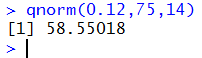
Thus, to find the value, X, for a population that is N(75,14)
we just need to use the command qnorm(0.12,mean=75, sd=14) as shown in
Figure 31.
Figure 31

As we have seen, having the named arguments mean=
and sd= in both pnorm() and qnorm()
can be quite convenient.
There does seem to be a little "overhead" in using them in the sense
that we seem to need to have to type the
mean=
and sd= as well as the values assigned to them.
In most cases this can be avoided because the formal definition of
the two functions gives these named parameters in
the second and third parameter position, respectively.
Figure 32 holds an excerpt from that formal definition.
Figure 32

In R, once named arguments have been assigned,
all unnamed arguments are assigned to the remaining
parameters in the order specified in the formal definition.
Therefore if we were to give the command
qnorm(0.12,75,14) the 0.12 is assigned to
q, the 75 is assigned to mean,
and the 14 is assigned to sd.
This more compact statement is shown in Figure 33.
Figure 33
Although this more compact form is available, it is my recommendation that you
stay with the longer named argument form of the commands.
If nothing else, it makes it much easier to check and confirm
your work.
Review for pnorm and qnorm
Listing of all R commands used on this page
x <- seq(-4, 4, length=200)
hx <- dnorm(x)
plot(x, hx, type="l", lty=1,
     xlim=c(-4,4), xaxp=c(-4,4,16),
     ylim=c(0,0.4), yaxp=c(0,0.4,8),
     las=2, cex.axis=0.75,
     xlab="z value",
     ylab="Density", main="Normal Distribution")
abline( v=0, lty=1, lwd=2)
abline( h=0, lty=1, lwd=2)
abline( h=seq(0.05,4,0.05), lty=3, col="darkgray")
abline( v=seq(-4,4,0.5), lty=3, col="darkgray")

plot(x, hx, type="l", lty=1,
     xlim=c(-4,4), xaxp=c(-4,4,16),
     ylim=c(0,8), yaxp=c(0,8,16),
     las=2, cex.axis=0.75,
     xlab="z value",
     ylab="Density", main="Normal Distribution")
abline( v=0, lty=1, lwd=2)
abline( h=0, lty=1, lwd=2)
abline( h=seq(0.5,16,0.5), lty=3, col="darkgray")
abline( v=seq(-4,4,0.5), lty=3, col="darkgray")

pnorm(-2.14)
pnorm(0.97)
1 - pnorm(0.97)

pnorm(0.97) - pnorm(-2.14)
pnorm(-2.14)+(1 - pnorm(0.97))

pnorm(0.97, lower.tail=FALSE)
# re-do P(X<-2.14) or P(X>0.97)
pnorm(-2.14)+pnorm(0.97,lower.tail=FALSE)

qnorm(0.05)

options(digits=13)
qnorm(0.05)
options(digits=7)

source("http://courses.wccnet.edu/~palay/math160r/gnrnd4.R")
gnrnd4( key1=121859504, key2=0002100345 )
L1
mu<-mean(L1)
mu
sd(L1)
pop_sd<-function( input_list )
{ n <- length( input_list)
sd( input_list )*sqrt((n-1)/n)
}
pop_sd( L1)
sigma<-pop_sd( L1)
sigma

summary(L1)

hist(L1,xlim=c(280,400),
     breaks=seq(280,400,5),
     xaxp=c(280,400,24),
     cex.axis=0.75, las=2, right=FALSE)

L2<-L1-mu
L2
mean(L2)
pop_sd( L2)
summary( L2)
hist(L2,xlim=c(-60,60),
     breaks=seq(-60,60,5),
     xaxp=c(-60,60,24),
     cex.axis=0.75, las=2)

L3<-L2/sigma
L3
mean(L3)
pop_sd(L3)
summary( L3)
hist(L3,xlim=c(-3,3),
     breaks=seq(-3,3,0.25),
     xaxp=c(-3,3,24),
     cex.axis=0.75, las=2)

pnorm(-0.8)

1-pnorm(2.5333)
pnorm(2.5333,lower.tail=FALSE)
pnorm(0.3333)-pnorm(-1)
1-(pnorm(1.2666)-pnorm(-0.4))

pnorm((138.5-100)/15)-pnorm((137.5-100)/15)

1-pnorm((137.5-100)/15)
pnorm((137.5-100)/15,lower.tail=FALSE)
pnorm((105.5-100)/15)-pnorm((84.5-100)/15)
1-(pnorm((118.5-100)/15)-pnorm((93.5-100)/15))

qnorm(.12)
qnorm(.12)*14+75

pnorm(83.4, mean=75, sd=14)
pnorm((83.4-75)/14)


1-pnorm(138,mean=100, sd=15)
pnorm(138,mean=100, sd=15,
      lower.tail=FALSE)
pnorm(105,mean=100, sd=15) -
      pnorm(85,mean=100, sd=15)
1-(pnorm(119,mean=100, sd=15) -
   pnorm(94,mean=100, sd=15))
#
#corrected to
#
1-pnorm(137.5,mean=100, sd=15)
pnorm(137.5,mean=100, sd=15,
      lower.tail=FALSE)
pnorm(105.5,mean=100, sd=15) -
      pnorm(84.5,mean=100, sd=15)
1-(pnorm(118.5,mean=100, sd=15) -
   pnorm(93.5,mean=100, sd=15))

qnorm(0.12,mean=75, sd=14)
qnorm(0.12,75,14)
Return to Topics page
©Roger M. Palay
Saline, MI 48176 December, 2015