This page will examine and step through multiple solutions
for hypothesis tests based on two samples
using the TI-83/84 calculators.
Figure 1
|
The standard error of the difference of the means is given by
`sqrt((s_1^2)/(n_1) + (s_2^2)/(n_2))`.
This would have been a pain to compute
had we not developed the CALCVSDF program in the last last chapter.
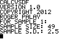
We start a run of the program here and give it the
sample size and standard deviation for the first sample.
|
Figure 2
 |
Figure 2 shows the completion of the data input for the program.
|
Figure 3
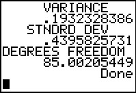 |
Figure 3 provides the output from the program. This gives us the standard
error as .4395825731 and the "complex" degrees of freedom as
B85.00205449.
|
Figure 4
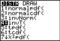 |
Because we do not know the standard deviations of the populations,
we use the standard deviation of the samples as our
estimate. Therefore, we are using the Student's-t
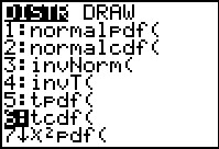
distribution. To get a "critical value" we can go to the
DIST menu and select invT(. [Note that users of
the TI-83, TI-83-Plus and early software for the 84-Plus can
use the INVT program to get the same values.]
|
Figure 5
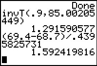 |
This is a one-sided test so our command is
invT(.9,85.00205449).
The result is our "critical value, 1.291590577.
The test statistic tht we want is
`t = ( (barx_1 - barx_2) - (mu_1 - mu_2) )/ sqrt((s_1^2)/(n_1) + (s_2^2)/(n_2))`
but under the null hypothesis `mu_1-mu_2` is zero. thus, we really calculate
`t = ( barx_1 - barx_2 )/ sqrt((s_1^2)/(n_1) + (s_2^2)/(n_2))` and we already have the value of that denominator.
Thus the command
(69.4-68.7)/.4395825731 will give us our test statistic.
The calculator produces the value 1.592419816.
This is more extreme than was our "critical value". Therefore,
using the "critical value" approach, we will
reject the null hypothesis in favor of the alternative hypothesis.
|
Figure 6
 |
To use the "P-value" approach we need to see how "extreme"
our test statistic turned out to be. TO do this we use the
tcdf( command, shown in Figure 6 in the DIST
menu.
|
Figure 7
 |
The result, computed with our "complex" degrees of freedom,
is .0575012782 which is less than the 0.10 given in
the problem. Therefore, this result is that we "reject" the null hypothesis.
|
Figure 8
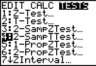 |
We just completed the problem by working it out using the
formula and variaous commands and programs. An alternative approach
is to have the calcualtor do all the work.
We find, in the STAT menu, under the TESTS sub-menu,
the item 2-SampTTest.... Choosing that
option opens a data input page.
|
Figure 9
 |
On this screen we have made sure that we are in the Stats
mode and that we have placed the appropriate values from the problem
into the fields of the screen.
|
Figure 10
 |
Moving down the screen we complete the settigns by choosing the
`>mu2` option. Then we highlight the Calculate option and
press  . .
|
Figure 11
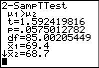 |
The result, shown in Figure 11, gives us both the appropraite
test statistic, namely t=1.592419816
and the P-value from that, namely
p=.0575012782.
These are the same values that we computed in Figures 1 through 7.
|
Use these data values to test the hypothesis `H_0: mu_1 = mu_2`
against `H_1: mu_1 > mu_2` at the 0.05 significance level.
Figure 12
 |
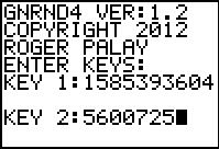
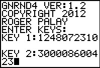
The first thing to do is to generate the data values.
As in earlier examples from the last chapter,
we will generate the second list
first and then copy to L2.
Figure 12 has the key values to generate the second table.
|
Figure 13
 |
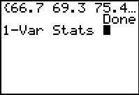
Figure 13 shows the start of the data, the command to copy
L1 to
L2,
and the command to find the one variable statistics
for the data.
|
Figure 14
 |
Figure 14 gives us the values that we need to be able to
follow the initial approach from the
previous example. In particualr, Figure 14
gives us the sample size, the sample mean,
and the sample standard deviation.
|
Figure 15
 |
Then we generate the first list of values.
|
Figure 16
 |
Again we see the start of that list and the command to get the one variables
statistics on that data.
|
Figure 17
 |
Now we have the sample size, sample mean,
and sample standard deviation from the second list.
At this point we are just where we were at the start of the
first example: we know all the needed values to do the
computation.
|
Figure 18
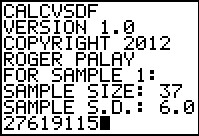 |
We use the information from Figure 17 to enter the
sample size and standard deviation into the CALCVSDF
program.
|
Figure 19
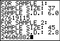 |
We complete the data entry for that program with
the information from Figure 14 for the second list.
|
Figure 20
 |
The program gives us the two values that we will need, namely, the
combined standard deviation 1.076684266 and the number
of degrees of freedom 48.87017928.
|
Figure 21
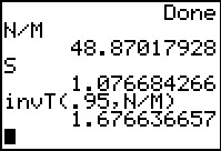 |
Before we go on to do the actual work here, we might recall that
the program stored the standard deviation in S and that
it found the degrees of freedom as the ratio N/M.
[One could look back at the program listing to confirm this.]
Therefore, when we ask for the value of S we get the
1.076684266 value, and when we ask for N/M
we get the 48.87017928 value.
We use this in forming the
invT(.95,N/M) command to get the "critical value" for this problem.
|
Figure 22
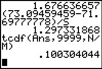 |
Again, following the earlier approach, we compute,
as we did in Figure 5,
the desired test statistic as the difference of
the sample means divided by the standard deviation.
However, in this case we shorten our typing
by using S for that standard deviation.
This gives us the test statistic as 1.297331868.
Using the "critical value" method, we note that this value is not
as extreme as was our critical value.
Therefore, we do not reject the null hypothesis, we accept it.
Alternatively, using the P-value method, we compute the
probability of getting a value as extreme or more extreme than the
one we got via the tcdf( command.
The result is .100304044, which is larger
than the allowed .05 given in the problem statement.
Again, we accept the null hypothesis.
|
Figure 23
 |
As with the first example, we really did not have to do all this work.
The calculator will do almost everything for us.
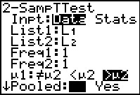
Figure 23 returns to the 2-SampTTest
input screen. GHere we have changed to the Data
option and we have given the names of the two lists holding
the sample data.
in addition, we have chosen the `>mu2` option.
|
Figure 24
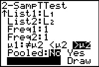 |
We move down to the Calculate option and press
.
|
Figure 25
 |
The calcualtor processes the two samples and
generates the screen shown in Figure 25.
This gives us the same values that we just computed the hard way.
|
Figure 26
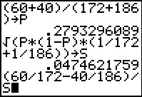 |
Unlike the process for finding confidence intervals,
the hypothesis test uses the pooled proportion
`hatp = (x_1 + x_2) / (n_1 + n_2)`.
Figure 26 shows the computation of that
value and storing it into P.
The desired standard deviation is then
` sqrt(( hatp*(1-hatp) )/(n_1) + ( hatp*(1-hatp) )/(n_2) ) = sqrt( hatp*(1-hatp)*(1/n_1 +1/n_2))`
which is also comptued in Figure 26 and stored in S
Finally, Figure 26 sets up the computation
of the appropriate test statistic.
|
Figure 27
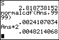 |
Figure 27 gives us the value of that test
statistic as 2.818738152.
We go on to find the probability of a
value this extreme or more extreme,
remembering that we are using a normal distribution.
Then, because this is a two-sided test,
we remember to multiply that result by
2 to get the total probability, namely, .0048214068.
This is less than the problem stated significance level of 0.005.
Therefore, we reject the null hypothesis in
favor of the alternative hypothesis.
|
Figure 28
 |
Alternatively, we could have used the calculator option
2-PropZTest... found tin the STAT menu
under the TESTS sub-menu.
|
Figure 29
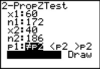 |
Figure 29 shows the resulting input form with
data from our problem supplied.
|
Figure 30
 |
Figrue 30 gives all the required results, identical to those we found
by our computations.
|
Figure 31
 |
Naturally, we start by generating the data.
|
Figure 32
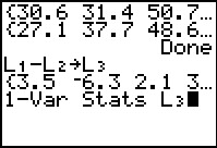 |
Once we have the data, we compute L3
as the difference of the paired values.
Then, we want to see the one variable statistics for
L3.
|
Figure 33
 |
Figure 33 gives us all the values we need.
|
Figure 34
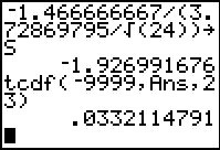 |
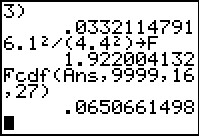
Our test statistic is the difference of the means divided by
the standard deviation of the mean of the differences.
But the difference of the original means is just the mean of the
differences, namely, -1.466666667 and the
standard deviation of the mean of the differences is
`3.72869795/sqrt(24)`.
We compute the desired quotient and store the result in
S.
Then we find the probability of getting a
value this extreme or more extreme.
using the student's-t distribution with 23 degrees of freedom,
this turns out to be .0332114791.
This is well below the given significance level of 0.100.
Therefore, we reject the null hypothesis in favor
of the alternative hypothesis.
|
Figure 34a
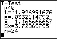 |
Alternatively, we could have gone back and selected the
T-Test option in the STAT menu, TESTS sub-menu,
told it that we want to process the data in
L3, set the test for ` |
We want to run a test on the null hypohtesis that
the standard deviations of two
populations are the same versus an alternative hypothesis.
We are given the following values:
Thus, we want to test `H_0: sigma_1 = sigma_2` against
`H_1: sigma_1 > sigma_2`, and do so at the 0.1 significance level.
This is a case where we have two data sets,
perhaps one from each of two treatments, and we want to test the
null hypothesis that the two populations have the same standard
deviation. In this example, we will test that against the alternative that
the standard deviation of the first is less than the standard deviation of
the second. We will set the level of significance at 0.100.
Figure 36
 |
The most straight forward way to do this is to generate the
two lists, obtain the statistics of each list,
pull out the necessary values, do the computation just as we did
in Figure 35.
As before, we start by generating the second list.
|
Figure 37
 |
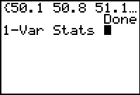
Once generated, we copy it to L2.
Then we ask for the 1-Var Stats.
|
Figure 38
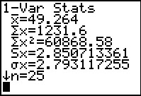 |
From Figure 38 we can get the sample size, 25,
and the sample standard deviation, 2.850713361.
|
Figure 39
 |
Now generate the first list.
|
Figure 40
 |
Ask for the 1-Var Stats.
|
Figure 41
 |
The first list has sample size of 27
and a standard deviation of
2.456672987.
|
Figure 42
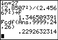 |
The test statistic is the quotient of the
two variances, with the large one in the numerator.
Figure 42 shows that this becomes 1.346509391.
Note that we had to use the variance of the second
list (even though we generated it first), as the numerator.
Therefore, the third parameter of the Fcmd( command
will be one less than the sample size of the second list,
or 24. That leaves one less than the sample size of the first
list, or 26, as the fourth parameter.
having formed and performed the command,
the result is .2292632314, a
value that is not less than the problem specified
significance level of 0.10.
Therefore, we accept the null hypothesis.
|
Figure 43
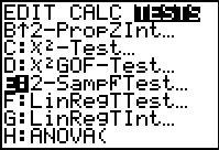 |
The computations that we just went through were
pretty straight forward. However, teh calculator
does have a command to do such a test. In the STAT menu,
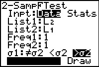
in the TESTS sub-menu, there is the 2-sampFTest....
|
Figure 44
 |
Figure 44 shows the input screen for that test.
The values for this problem have been given.
We can go ahead and perform the test.
|
Figure 45
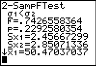 |
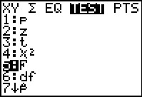
The result is shown in Figure 45.
However, there is a problem here. Indeed, the
resulting probability, .2292632314, is just what we
computed in Figure 42. As such, we will still accept the null hypothesis.
But the F statistic is all wrong. Figure 45 gives it as
.7426558364. Not only is this different from the
1.346509391 we computed above, but it is less than 1.
This seems impossible given that our quotient has the larger
variance in the numerator.
What is wrong?
|
Figure 46
 |
In order to help find the problem, we will first find the
variable that the calculator uses to hold the F statistic.
We find it in the VARS, Statistics, TEST menu.
|
Figure 47
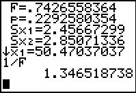 |
In Figure 47 we have used that variable to get 1/F.
This turns out to be exactly the value that we thought we would get
for the F statistic.
It seems that the calcualtor has computed the
quotient, but done so with the numerator and denominator reversed.
It appears that the calculator uses the List1: list in the numerator
and the List2:
list in the denominator. Just looking at the two original lists
we do not realize that the second list has the larger variance.
Looking at the results that we obtained in
Figures 38 and 41 we see that this is indeed the case.
|
Figure 48
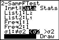 |
Perhaps the solution is to reverse the order of the two lists in the
input screen. In Figure 48 we have done that.
Now we can try again.
|
Figure 49
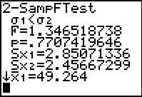 |
These results are different, but they still pose a problem.
Now the F statistic is correct, but the probability is wrong.
The new probability is just 1-.2292632314.
This should lead us to understand that
we reversed the the two lists but we did not reverse the
direction of the alternative. The original alternative
was `sigma_1List1: is L1
and List2: is L2.
However, in Figure 48 we reversed this. Therefore we need to
reverse the alternative and make it `sigma_1>sigma_2`.
|
Figure 50
 |
Figrue 50 shows that change.
|
Figure 51
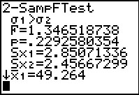 |
Figure 51 shows the results. We finally have the right answers.
The lesson here is that
the calculator does its thing the way it wants to.
We can use the approach shown in Figures 36 through 42
and get pretty clear results.
Alternatively, we can use the 2-SampFTest process
but we better be ready to change our input
to get the desired output.
|