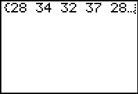
We need to start with some data. We will generate a list of data on the calculator using GNRND4 with Key 1=131425002 and Key 2=1100026. That list will be the same numbers that appear in the following table: Thus, our problem will be to generate a frequency table for the data in the list above.

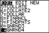
Figure 1	We begin by getting the data into the calculator. We could do this by entering each of the 51 values into the calculator. This, however, is prone to error. A better way is to take the option of running the GNRND4 program. We need to start the GNRND4 program. To do this we open the Program Menu by pressing the key. The resulting screen start the list of programs that are on the calculator being used. In this case, the calculator has quite a few programs, enough so that we cannot see the desired GNRND4. Therefore, we use the key to move down the list.
Figure 2	In Figure 2 we have found the GNRND4 program. It is beyond the numbered positions. However, since it is the program selected by the cursor, we can press the key to cause the program command to appear on the main screen, as shown in Figure 3.
Figure 3	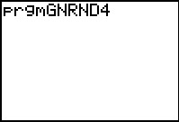Notice that the calculator has automatically placed the characters "prgm" before the name of the program we want to run. All that remains now is to press the key again to start the program.
Figure 4	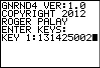The program starts by displaying some vital information. Then the program prompts for the Key 1 value. In the example we are using we need to enter 131425002 in response to that prompt. Figure 4 shows the screen after we have entered that value. Then we press the to continue the program.
Figure 5	Now GNRND4 is asking for the second key value: we respond with the value 1100026. Then we press the to continue the program.
Figure 6	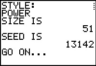As shown in Figure 6, the GNRND4 program then displays some data about the process it is running. The pargram then waits in a "pause" state, for us to press the key in order to continue.
Figure 7	Continuing, the program displays more data, again waiting for us to press the to go forward.
Figure 8	After Figure 7 and before Figure 8, the calculator displays a screen that slowly fills with dots. That screen, which I cannot capture so that I can display it here, just lets you know that the calculator is continuing to work on the task. Once the task is completed, the calculator erases the screen of dots and displays the list of values that has been generated. Figure 8 shows this list. The calcualtor is in a "pause" state (note the pattern of dots in the upper right corner of the screen). This allows us to use the left and right cursor keys to move through the entire list.
Figure 9	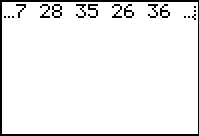To move from Figure 8 to Figure 9 we have used the key a number of times. Note that starting in Figure 8 and continuing in Figure 9, the numbers in our list are identical to the numbers given in the table above.
Figure 10	For Figure 10 we have pressed the key again and again to move to the very end of the list. Here we can see that the end of the list corresponds to the end of the values in the table above. Note that the program is still "running" although it continues to be in the "pause" state. To finish the program we need only press the key.
Figure 11	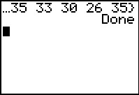Figure 11 shows that the program has completed. We can no longer scroll through the values in our list. However, the list that was generated in stored in the calculator in L1.
Figure 12	One way to examine the contents of L1 is to use the STAT editor. To get to this we press the key to bring up the display shown in Figure 12. The option that we want to select from this is the first one, Edit..., and its number, 1 is already highlighted. Therefore, we can either press the key or the key to start that option.
Figure 13	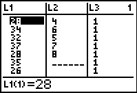Figure 13 shows the Editor. We are interested in examining L1. (The calculator used here had some previous use for L2 and L3, but we ae not concerned about those values.) Figure 13 shows the first 7 items in L1, along with not only highlighting the first item but also making a specific reference to it at the bottom of the screen. We can use the and keys to move through the items in L1.
Figure 14	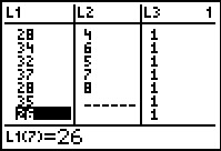For Figure 14 we have moved the highlight to the seventh item in L1. We can continue using the key to display more items in the list. In this case, we will use that key to move all the way to the bottom of the list, shown in Figure 15.
Figure 15	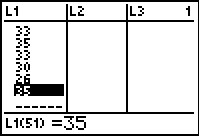Here we are at the end of the list. Again we can compare the numbers in the list to those in the original table of values given above to verify that we have exactly the same values. To get out of the Editor we use the key sequence . This will return us to the screen shown in Figure 16.
Figure 16	Having seen the list of values in L1, we are ready to start working with that list in order to produce a frequency table. The approach here will be to sort all of the values so that we can merely move through the list, observing each different value and counting the number of times each different value is in the list. To sort the list into ascending order we need to get to the SortA( command. We will find that command in the LIST menu, and we get to that menu via the key sequence .
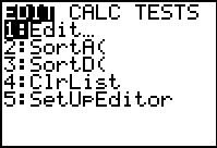
Figure 17	Figure 17 shows the LIST menu, or rather, the NAMES sub-menu of the LIST menu. We could use this sub-menu to select a name of a list that is defined on this calculator. The option that we want is in a different sub-menu, in particular, it is in the OPS sub-menu. To get there we use the key. Moving us to Figure 18.
Figure 18	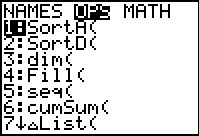Figure 18 shows the OPS sub-menu. We have the desired SortA( option here. Since that is the option that is highlighted, we select that option by pressing the key.
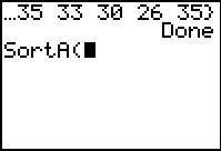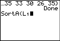
Figure 19	Having selected the option, the command SortA( has been pasted onto our screen. We need to give the calculator the name of the list to sort into ascending order. We can specify the L1 list by using the key sequence .
Figure 20	Now the command is almost complete. We can press the key to add the closing right parenthesis, shown in Figure 21.
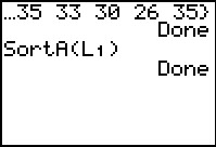
Figure 21	Having completed the command, we press the to perform the cammand. The calculator does the work and signals that it has completed the work by displaying Done. We want to return to examine the resulting sorted list. To do that we return to the STAT menu by pressing the key.
Figure 22	To start the Editor we press the key.
Figure 23	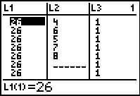We can see here that the values in L1 have been sorted. In fact, we can see that the lowest value is 26. Now we want to know how many 26's are in the list. We use the key to move down the list, looking for the next different value.
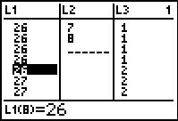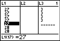
Figure 24	Figure 24 shows that we have found a new value, namely, 27 at position 9. Therefore, we know that we have 8 26's. We could start our Frequency table with this information: Value Frequency 26 8 27
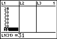
Figure 25	We left Figure 24 knowing that the next value is 27. We move further down the list to see what follows 27. In Figure 25 we see that the last 27 is in postion 17. Thus, we have 9 such values. We can modify our table to be: Value Frequency 26 8 27 9 28
Figure 26	Moving further down the table we see that we have 6 28's and 2 29. Thus we update the table to Value Frequency 26 8 27 9 28 6 29 2 30
Figure 27	There are 5 30's.
Figure 28	There are 2 31's and 1 32.
Figure 29	There are 5 33's. Our table has grown to Value Frequency 26 8 27 9 28 6 29 2 30 5 31 2 32 1 33 5 34
Figure 30	There are 3 34's.
Figure 31	There are 4 35's.
Figure 32	There are 3 36's.
Figure 33	And there are 3 37's. (We recall that there are 51 items in the list. We saw this in Figure 6 and in Figure 15. We could move down one more to verify that we are at the end of the list if we wanted to do that.) Our final table becomes Value Frequency 26 8 27 9 28 6 29 2 30 5 31 2 32 1 33 5 34 3 35 4 36 3 37 3
Figure 34	We created the data in Figures 1 through 16. We used a brute srength and awkwardness approach to process the data in Figures 17 through 33. The next section of this page gives an alternative approach to that analysis of the data. We will run the COLLATE2 program to mimic and add to the work we have done above. First we open the program menu via the key. We see that the program we want is in position 6 of this listing. We can select that option by pressing the "6" on the keypad. However, we happen to know that the COLLATE2 program requires that the TOSTR2 program be on the calculator. (COLLATE2 calls TOSTR2 as a subroutine.) In order to verify that the TOSTR2 program is loaded we use the to scroll down the list of programs.
Figure 35	Figure 35 shows that the TOSTR2 program is in fact present. Even though the COLLATE2 program is not on the screen at the moment we know that on this calculator the COLLATE2 program is currently in position 6 in the list of programs. Therefore, on this calculator, at this time, we can select that 6thoption by pressing the key now.
Figure 36	The result of that action is to paste the command prgmCOLLATE2 on the screen, as is shown in Figure 36.
Figure 37	We press to start the program. The program clears the screen and prompts us for the name of the list holding the values. [Please note that Figure 37 shows the output from Version 2 of the COLLATE2 program.)
Figure 38	The list of values that we want to use is in L1. We enter that name via the key sequence . This enters the name at the end of the prompt, as is shown in Figue 38. From there we press to have the calculator continue with the program.
Figure 39	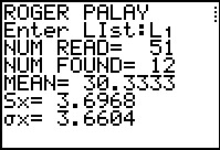Figure 39 shows some of the output for the program. Note that it gives the number of items in the list, and the number of different items in the list, as well as some additional data. The program goes into a pause state at this point, waiting for us to press to continue.
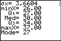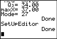
Figure 40	Figure 40 gives the rest of the output from the program. This has two pieces of information that are helpful to our current task, namely, the low value (in this case 26) and the high value (in this case 37). Again, noting the dots in the upper right corner, the program is in a paused state. We can complete the program by using the key.
Figure 41	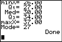The program has finished its work and it displays the Done in Figure 41. Now, besides producing the output shown in Figures 39 and 40, COLLATE2 also creates some new lists and the program changes the STAT Editor to display these new lists.
Figure 42	To get to the STAT Editor we open the STAT menu via the key. Then we press the key to start the editor.
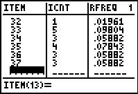
Figure 43	Comparing Figure 43 with Figure 23, we see that there are different lists being shown. These new lists we created by the COLLATE2 program and they were put into the STAT Editor by that same program. ITEM, the first list, gives the different values that were in the original data list. In effect, ITEM holds the first column of our frequency table, the column giving the values found. Compare the conents of ITEM with the first column of the frequency table shown above with Figure 33. ICNT, meaning Item Count, holds the number of times each different ITEM value was found. This is the "frequency" column of our frequency table. Aga9n, compare the values under ICNT tot he values in the table to the right of Figure 33. COLLATE2 has done our work for us. We do recognize that we will need to use the key to move down the editor to see the other values for our table. This is shown in Figure 44.
Figure 44	Here we see the remaining values and frequencies that we need to use. To exit this screen we use the key sequence. That will return us to the main screen. One additional activity for us will be to return the Stat Editor to its default display. To do this we press the key to open the STAT menu, shown in Figure 45.
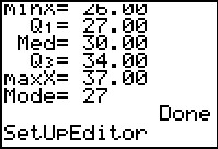
Figure 45	Here we see the STAT menu, and we have moved the highlight down to the SetUpEditor option. We press the to paste tht option back onto the main screen.
Figure 46	having pasted the command here, we press to perform the command. This command, without any additional lists being noted, will restor the default setting for the Editor.
Figure 47	The calculator has let us know that the command has been performed. We can verify this by first returning to the STAT menu via the key.
Figure 48	Then, prssing the key will open the Editor, as shown in Figure 49.
Figure 49	We can see that the Editor has been returned to displaying the built-in Lists. We can exit this via the key sequence.
Figure 50	The following Figures demonstrate using the calculator with some degree of finess to achieve the same results that we found first by brute strength and awkwardness, and tehn via the COLLATE2 program. In particular, we will use the built-in feature of the calculator that produces histograms of data, and we will force that display to give us the frequency of our values. We start by moving to the STAT PLOT menu via the key sequence
Figure 51	The particular calculator used here already had Plot1 turned on. We want Plot1 turned on, but we also want to change a different setting for Plot1. In order to make changes to the Plot1 values we press the key.
Figure 52	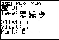In Figure 52 we see the options for Plot1. In particular, the plot is "On", the type is set to a "scatter plot", and that scatter plot will be of x-values stored in L1 and corresponding y-values stored in L2, with the points of the plot marked by small squares. [Had Plot1 been turned "Off" we could have turned it "On" by highlighting the "On" and pressing the key. Since Plot1 is already "On" we will leave it alone.] We want to change Plot1 to be a "histogram", the third Type in the first row of Type options. Using the cursor keys we will move the highlight to that option.
Figure 53	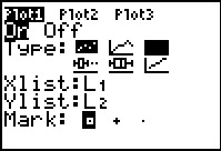In Figure 53 we have moved the highlight to the desired option. In this case we have captured the screen image as the blinking cursor was in its all-black mode. To change the selection to this option we press the key.
Figure 54	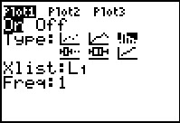Figure 54 shows that we have indeed changed the Type option. Note that this also changed the rest of the screen so that the histogram will now be based on the data in L1 and our grouping for the height of each bar in the histogram will be 1. We have set up Plot1 the way we want it. We can jump to the ZOOM menu by pressing the key.
Figure 55	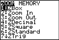We have jumped to the ZZOOM menu because we want to use the ZoomStat option. We want to use this option because it will set the WINDOW values according to the data that is in our list. However, as you can see, ZoomStat is not displayed on this screen. Instead we will need to use the cursor keys to move down the menu to find ZoomStat.
Figure 56	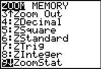Here we have found ZoomStat in the menu and we have left it highlighted. Thus, to perform the option we need only press the key.
Figure 57	The result is the accurate histogram shown in Figure 57. This is a correct histogram but it is not the one we want. We notice that it has 8 classes and we want 12. The problem is that the ZoomStat option forced the calculator to make some choices on the width of the classes as well as on the lower and upper limits on those classes. We want to revise that choice. To do this we press the key to open the WINDOW menu.
Figure 58	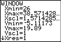Figure 58 shows the WINDOW values established by the data we have and the default attempts of the calculator brought into play by the ZoomStat option. We want to revise these settings so that each class will hold one and only one of our 12 different values. Our changes are shown in Figure 59.
Figure 59	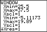Now we have classes that are 1 unit wide, with the first class starting at 25.5 and therefore ending just before 26.5. That class will hold any of our values that fall in that range, which means that all of the 26's will fall in this class, and none of our other values will be in this class. We return to see a new historgram by pressing the key.
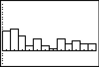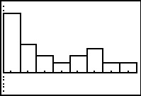
Figure 60	Figure 60 holds our revised histogram and it does have the 12 classes that we desired. We would like to know the height of each of the rectangles because that height will be the frequency of the value that the particular rectangle represents. To see the height of each rectangle we will move into TRACE mode by pressing the key, after which we see the information shown in Figure 61.
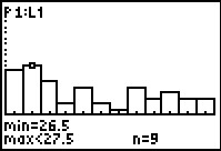
Figure 61	Now that we are in TRACE mode, the display in Figure 61 shows that for the first rectangle on the graph, the rectangle represents values from 25.5 to 26.5, and that there were 8 values in our original data that fell into that range. Since the only value in our original data that falls into this range is 26, we now know that the frequency of the B26's is 8.
Figure 62	In Figure 62 we have used the key to move opur trace to the next rectangle. The range for this rectangle is values from 26.5 to 27.5, and there were 9 such values. Thus, the frequency of the 27's is 9. We can keep moving across the various rectangles to get a frequency for each of the values in our original table, and from this we could generate the same frequency table that we constructed back in Figure 29.
Figure 63	Just to wrap up the display, Figure 63 shows the range and the count (frequency) for the final, rightmost, rectangle on the histogram.