This page will look at the F distribution and its use in a hypothesis test of the equality of two standard deviations. To start, consider the following three points:

1. The normal distribution, for mean=0 and standard deviation=1, is well defined. Almost all of the area under the normal distribution function is contained between –3.99 and 3.99. As such, we can construct a single, relatively small, table that gives the area to the left of any z-value between –3.99 and 3.99. Furthermore, we can use that one table to either read the area given a z-score or to find the required z-score given the area value.
2. The Student's t distribution, for mean=0 and standard deviation=1, is defined based upon knowing the number of degrees of freedom. That is, the Student's t distribution has a different table for each number of degrees of freedom. Although it is reasonable to post such tables on a web page, as we have seen starting from an Index of Student t tables page, including so many tables in a statistics book would be unwieldy. Instead, in a statistics book we generally find a table that just gives selected critical points in the Student's t distribution for various degrees of freedom and for predetermined areas of interest, as we saw on the page Critical Values of Student's t page.
3. The F distribution is based on a ratio of variances. Therefore, the possible F values are
   1. are all positive (being the quotient of positive values);
   2. would be 1 if the variances were equal;
   3. if the first variance is 7 and the second is 3, then the quotient is 7/3 or approximately 2.3333;
   4. if the first variance is 3 and the second is 7, then the quotient is 3/7 or approximately 0.2857.
   5. the F value will be dependent upon both the degrees of freedom of the numerator and the degrees of freedom of the denominator.
   The first consequence of these points is that if we were to generate F distribution tables, as we did as web pages for the Student's t distribution, then we woud need a different table for each possible combination of the degrees of freedom for the numerator and the degrees of freedom for the denominator. A second consequence is that the F values for situations where the numerator is larger than the denominator would increase from 1 to possibly huge values, whereas, the corresponding situation where the numerator is smaller than the denominator would be crammed into the range between 0 and 1. Therefore, textbooks adopt a scheme similar to that of the Student's t in that books generally provide two, or even three, separate tables of critical values, one table for a given area of interest and all of the pairs of numerator and denominator degrees of freedom. Furthermore, since any problem where the numerator variance is less than the denominator variance can be recast, restated, so that the numerator variance is greater than the denominator variance, the tables provided in the textbooks cover only the latter case.

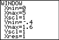
Figure 1	Before we look at the F distribution, we open the WINDOW menu and set the values as indicated in Figure 1. Note that the X values will run from 0 to 5.
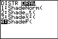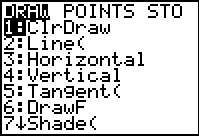
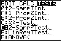
Figure 1a	Then use the sequence to open the DIST menu and use the key to move to the DRAW submenu shown in Figure 1a. Once there we have used the key to move the highlight to the ShadeF( option. Press to move to Figure 2.
Figure 2	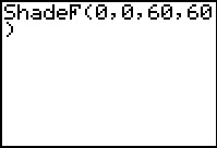Figure 2 shows the completeed command that we started in Figure 1a. The command tells the calculator to draw the F distribution, shading everything from 0 to 0 (i.e., do not shade anything), for 60 degrees of freedom for the numerator and 60 degrees of freedom for the denominator. Press to perform the command.
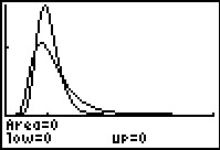
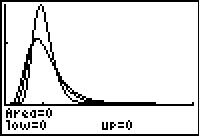
Figure 3	It actually takes quite a while for the calculator to draw the curve shown in Figure 3. The calculator is not done until it writes the information at the bottom of the screen. Remember that the total area under the curve is equal to 1 square unit. Also, the Y-scale goes up to 1.6 and the X-scale goes from 0 to 5. We can see that the curve is skewed to the right (the long tail). Also, almost all of the area is between 0.4 and 2.2. [Indeed, it is the computation of all of the points from 2.2 to 5.0, points that end up being rounded onto the x-axis, that caused the calculator to look like it was doing nothing for so long.] Having seen the F distribution with degrees of freedom equal to 60 and 60, let us look at how the graph changes if we alter the degrees of freedom.
Figure 4	To do this we create another ShadeF( command. We can do this by retracing our prvious steps or by using the key sequence to recall our previous command and then use the cursor keys to help edit that command. For this new command, shown in Figure 4, we have set the degrees of freedom for the denominator to be 15. Press to perform the command.
Figure 5	The new drawing is superimposed on the previous one. The new curve is more spread out than was the first. There is more area under the curve closer to 0 and more area under the new curve further to the right. We still see that there is hardly any area under the curve to the far right.
Figure 6	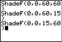Next we recreate or recall the ShadeF( command, but this time we reverse the degrees of freedom for the numerator and denominator. In this new command we want 15 degrees of freedom for the numerator and 60 degrrees of freedom for the denominator. Press to perform the command.
Figure 7	In Figure 7 we see all three curves. We can see that these are three distinct curves. The curves for Shadef(0,0,60,15) and the ShadeF(0,0,15,60), though distinct, are really quite similar.
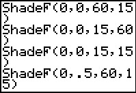
Figure 8	For completeness, we will construct yet a fourth curve, namely ShadeF(0,0,15,15).
Figure 9	The new curve is even more flattened out, having still more area to the left and to the right under the curve.
Figure 10	As we have seen, drawing repeated images merely superimposes those images. We can clear the display by using to open the DRAW menu. From there we select the ClrDraw command.
Figure 11	As a result we have a clear drawing, as shown in Figure 11.
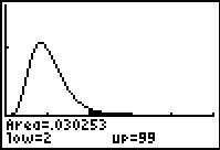
Figure 12	To get an idea of the area under the curve, we return to the ShadeF( command. This time we will ask the calculator to shade under the portion of the curve from 0 to 0.5 for the case where the numerator degrees of freedom is 60 and the denominator degrees of freedom is 15.
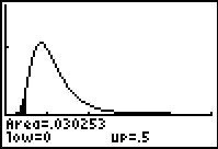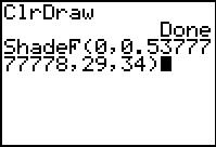
Figure 13	Figure 13 not only shows that shading but also gives the value of that area as 0.030253. Before leaving Figure 13 we return to the Draw menu and again clear the display.
Figure 14	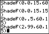In the points presented above we noted that if the ratio of the variances is 0.5, then we can restate the problem to reverse that fraction, in which case we get 2.0. Let us construct the shaded area under the curve from 2.0 to 99. The command ShadeF(2,99,60,15) would seem to do this. Perform that command to generate the curve in Figure 15.
Figure 15	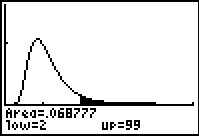As expected, the area under the curve, from 2 up to 99 (only up to 5 is shown on the graph), is shaded in Figure 15. What we did not expect is that there is a different amount of area on this right side as compared to the area we found on the left side back in Figure 13. The difference in values is a result of our overlooking the required change in the degrees of freedom. The original, Figures 12 and 13, graph had a ratio of the variances as .5, but that was from having the numerator with 60 degrees of freedom and the denominator with 15 degrees of freedom. If we invert the ratio, then we must have the new numerator (i.e., the old denominator) set to 15 degreees of freedom and the new denominator (the old numerator) set to 60 degrees of freedom.
Figure 16	As before, we will ClrDraw and then recreate (or recall and edit) the ShadeF( command to correctly associate the degrees of freedom with the appropriate numerator and denominator.
Figure 17	Finally, in Figure 17, we see the "flipped" verson of the problem from Figure 13. We see that the calculator has again determined that the shaded area is 0.030353, just as it was, on the left, in Figure 13.

Let us see how all of this works when we have a real problem. We are given the following data related to two samples:

Figure 18	We will start this problem using the 2-SampFTest found in the STAT menu under the TESTS tab as shown in Figure 18.
Figure 19	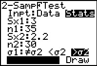The 2-SampFTest allows us to enter the actual "statistics" for our problem. In Figure 19 we have specified the standard deviations and size of the two samples. We have also set the appropriate alternative hypothesis. Having highlighted the Calculate field we press to have the calculator perform the test.
Figure 20	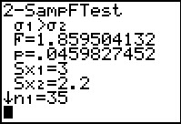Figure 20 gives the result of the test. In particular, the calculator repeats the alternative hypothesis `sigma_1>sigma_2`, it gives the F-statistic, namely 1.859504132 (which is exactly the value of `(s_A^2)/(s_B^2)=(3^2)/(2.2^2)=9/4.84`), and it gives us the attained probability as `0.0459827452`. The display goes on to echo the standard deviations and sample sizes that we used. We should note that behind the scenes this test computed the area under the F distribution curve for 34 and 29 degrees of freedom to the right of the value 1.859504132. We can see that in the following Figures.
Figure 20a	In Figure 20a we have formulated exactly the request that will graph the F distribution for 34 and 29 degrees of freedom, and shade the area under the curve to the right of the value 1.859504132.
Figure 20b	Figure 20b shows the graph and it also gives the area of the shaded region as 0.04593, just what we expected.

We should pause here to note that if we were doing this problem using the tables in a book, then we could look at the table that gives critical values for the F distribution, specifically for the 0.05 significance level, to find out the critical F value associated with 34 and 29 degrees of freedom. This often entails a bit of interpolation. For example, in a statistics text I found a table that gives the following values:

Now that we have looked at this problem, let us go back and ask the question what would have happened if the origianl data had been given as:

To do this test on the calculator we follow exactly the same steps that we took in the first version of the problem, back in Figures 18 through 20.

Figure 21	In Figure 21 we have set up the problem, making sure that we have the values in the right place and that the alternative hypothesis is the approptiate <σ2. We press to perform the test.
Figure 22	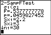The F value has been computed as 0.5377777778, which is the value of `(2.2^2)/(3^2)`. The attained significance is 0.459827452, exactly as we found in Figure 20. This time, because we have the lower standard deviation in the numerator, our F value will be a number less than 1. The more extreme values will be values further from 1, and, since the values need to be positive, closer to 0. The calculator understands this and we can just use the attained significance to determine that we reject the null hypothesis at the 0.05 level because the attained significance is less than that level.
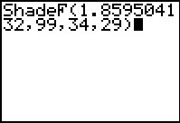
Figure 22a	We can use the ShadeF( command to get a picture of the area to the left of the computer F value, that is, the area associated with values more extreme than that value. Figure 22a shows the formation of such a command. Note that we have to have the correct order for the degrees of freedom. This order reflects the fact that the sample C value is in the numerator while the sample D value is in the denominator of our computation of the F value.
Figure 22b	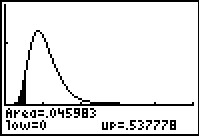And, indeed, Figure 22b shows the area in the left tail of the distribution, the area to the left of 0.5377777778. This figure also shows that the attained significance is 0.045983.

Having used the calculator to do this problem we might consider trying to do it with the tables for the F distribution that we find in statistics text books. However, we cannot do this. The tables in standard books for the F distribution only give values for the right tail That is, we cannot directly use those tables to find a critical F value that has a significance of 0.05 for the left tail given 29 and 34 degrees of freedom. This shortcoming give rise to the requirement, if we are going to use the tables, that we state the problem in such a way that the larger sample variance is in the numerator and the smaller is in the denominator. In such a case we will have the computed F value be greater than 1 and the more extreme F values will be those that are even larger than the computed value. Fortunately, there is a simple conversion from the F value we found in Figure 22, namely, 0.5377777778, to the associated F value that is greater than 1.

Figure 23	To make this conversion we have to find the multiplicative inverse of our F value. That is we can compute `1/F` or `F^(-1)`. In Figure 23 we have moved to the VARS menu. From there we select the Statistics... option to move to Figure 24.
Figure 24	In the Statistics option we move to the TEST tab. There we see the variable F. Once highlighted, we can press the key to paste that variable onto our home screen.
Figure 25	We complete the command by pressing the key to generate our desired `F^(-1)`. Then press to have the calculator perform the command. In this case the value is the expected 1.859504132, the same value that we saw when we had stated the problem originally, back in Figures 18 through 20b.

We have seen how to perform our test if we have the statistcs for the samples. Let us consider the case where we have two samples.

We have two data sets, perhaps one from each of two treatments, and we want to test the null hypothesis that the two populations have the same standard deviation. In this example, we will test that against the alternative that the standard deviation of the first is less than the standard deviation of the second. We will set the level of significance at 0.05.

As we have seen in previous examples on previous pages, because the GNRND4 program always produces its values in L₁, if we are going to keep the data in a convenient order, that is, we want the first data list in L₁ and the second in L₂, then we will start by generating the second list and then we will copy it to L₂ before we generate the first list in L₁.

Figure 26	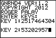In Figure 26 we have started the GNRND4 program, giving it the specified key values for the second data list.
Figure 27	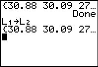Figure 27 shows not only the completion of the GNRND4 program but also the command to copy L1 to L2. Once that is done we are free to generate the first data list starting in Figure 28.
Figure 28	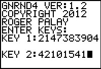Here we have started the GNRND4 program again, this time giving it the keys for data set 1.
Figure 29	Figure 29 shows the completion of the program. Our data is now in the calculator.
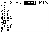
Figure 30	We return to the STAT menu, select the TEST tab, and then select the 2-SampFTest option to get to Figure 30. On this screen we tell the calculator that we do have the Data, that the first list is in L1, that the second list is in L2, (these are lists of the actual data where each item in the list is treated as appearing one time so we leave the Freq values at 1) and we specify that the alternative hypothesis is `sigma_1` < `sigma_2`. Then we have the calculator Calculate the test values.
Figure 31	Because the calculator does not use the limited tables found in text books, the calculator has no need to make sure that when it forms the F value that it uses the larger of the two variances as the numerator. In the case we see here the larger value is for the second data list. The calculator always forms the the F value by taking the quotient as the first list variance divided by the second list variance. Therefore, the F value is computed as 0.5536628241. The more extreme values will be those less than that F value. The attained significance of 0.032222916 is less than our given level of significance, 0.05, so we will reject the null hypothesis in favor of the alternative hypothesis.
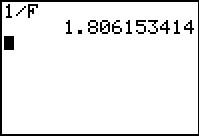
Figure 32	Were we doing this using tables, we would need to compute the F value by having the larger variance in the numerator of the quotient. We can find that value here by evaluating 1/F where we find the F variable in the VARS menu, Statistics option, TEST tab. We see that the value is 1.806153414. We would then have to use the tables to find, for a 0.05 level of significance, the critical value for 43 and 40 degrees of freedom. Note that we had to use the sample size of the second data list as the numerator degrees of freedom because we are using the variance of the second data list as the numerator of the F value. Furthermore, our extreme values would now be values to the right of the critical value because we are now \really looking at an alternative hypothesis that could be stated as `sigma_2` > `sigma_1`. This is mathematically equivalent to the original alternative hypothesis, but it allows us to use the tables because the fraction is now greater than 1.
Figure 33	Of course, we could also do this right in the calculator. In Figure 33 we have returned to the 2-SampFTest screen where we have changed the place of L1 and L2 and we have appropriately changed the selection of the alternative hypothesis.
Figure 34	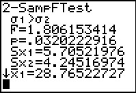We see the results in Figure 34. The F value is now our expected 1.806153414 but our attained significance is the same 0.0320222916.