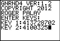
We will generate a list of data on the calculator, using
GNRND4 with Key 1=413728702 and Key 2=4100325. That list
will be the same numbers that appear in the following table:
Thus, our problem will be to generate a dot plot diagram for the data in the
list above.
Figure 1
|
We start with a run of the GNRND4 program,
giving the program the specified key values.
Press  to continue. to continue.
|
Figure 2
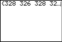 |
After skipping over two intermediate screens, the program displays the
generated values. These are the same as the values shown above.
The program saves these values in the list L1.
Again, press to finish the program.
|
Figure 3
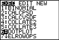 |
We return to the list of programs via the  key. Then
use teh key. Then
use teh  key to move the highlight
down to the DOTPLOT program. Press
to select that choice. key to move the highlight
down to the DOTPLOT program. Press
to select that choice.
|
Figure 4
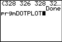 |
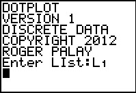
The command prgmDOTPLOT is pasted on the main screen.
Press to perform that command, i.e., run
the program.
|
Figure 5
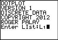 |
The program starts with information about itself, and then it asks for
the location of the data to use. We respond with
  to indicate that the data is in L1.
Then press to continue the program.
to indicate that the data is in L1.
Then press to continue the program.
|
Figure 6
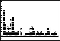 |
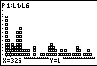
The DOTPLOT program does some more computations and then it finally
displays the dot plot as shown in Figure 6.
Although the plot is accurate, it is a bit confusing in that we have no idea, from the plot, about the values being represented.
One way to try to find out some of those values is to move into Trace mode.
Press the  key to move to Figure 7. key to move to Figure 7.
|
Figure 7
 |
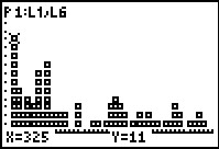
Now we are in trace mode. The claculator has highlighted (although it is almost impossible to see this) the first point being plotted.
Furthermore, the calculator is displaying the cooordinates of that point, namely (325,1).
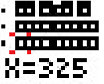
The highlighted point is in the lower left corner of the plot. The
highlight amounts to four little dots surrounding the
point. Here is a magnification of the lower left corner with those dots displayed in red.
|
Figure 8
 |
If we use the  key repeatedly we can move that highlight to subsequent points on the
plot. In Figure 8 we have moved to highlight the eleventh point, the one at the top
of the first column. Its coordinates are (324,11). key repeatedly we can move that highlight to subsequent points on the
plot. In Figure 8 we have moved to highlight the eleventh point, the one at the top
of the first column. Its coordinates are (324,11).
|
Figure 9
 |
Using one more time moves the highlight to the twelfth point,
the lowest one
in the second column. Its coordinate is (326,1).
|
Figure 10
 |
We can exit the plot by using the sequence
 .
This takes us back to the main screen. .
This takes us back to the main screen.
|
Figure 11
 |
We want to see some of the background processing for DOTPLOT.
We know that the data was in L1.
We move to the STAT menu via the  key.
Then press to open the Stat editor
show in Figure 12. key.
Then press to open the Stat editor
show in Figure 12.
|
Figure 12
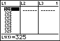 |
It is pretty clear that the DOTPLOT program sorted the values in L1.
We can use the key to move down the list to inspect more values.
|
Figure 13
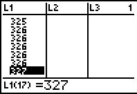 |
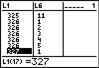
To get to Figure 13 we have moved down the list to highlight the 17th
item (Note the L1(17)=327 at the bottom of the screen.) At the top of the list we see the final 325 point.
Then there are five 326 values. Then we start the 327 values. However, nothing appears in the
other lists being displayed. Were we to look at a listing of the DOTPLOT
program, we would find that the program uses
L1 aned L6.
We can move to the right, using the
key, to look at L6.
|
Figure 14
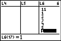 |
For Figure 14 not only have we moved to display L6
but also we have moved down the list to highlight the
17th item in that list. Thus, Figure 14 parallels Figure 13.
In L6 we are seeing the second coordinate for each of the plotted points.
This would be easier to see if we could display L1
and L6 side-by-side.
We will cause this to happen.
|
Figure 15
 |
Use
to exit Figure 14 and return to the main screen.
|
Figure 16
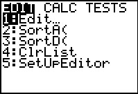 |
Use to open the STAT menu.
From that menu select the fifth
option by pressing the  key. key.
|
Figure 17
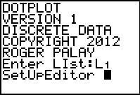 |
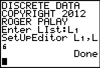
That action caused the SetUpEditor command to be pasted onto the main screen.
|
Figure 18
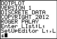 |
We will append L1,L2
to this via the key sequence

 .
Then press to move to Figure 19. .
Then press to move to Figure 19.
|
Figure 19
 |
Here we see that the calculator has told us that it has completed the command.
Now return to the STAT menu via the
key and move to the editor via the key.
|
Figure 20
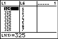 |
Figure 20 show us the two lists, side-by-side, as we had wanted.
|
Figure 21
 |
For Figure 21 we have moved down the lists so that we can see the 17th
item at the bottom. Now it is easy to see the correspondence between the
values in L1 and L6
as being the coordinates of the points plotted on the graph.
|