For both correlation and regression we assume that we are dealing with data that is given as pairs of values, an X value and a corresponding Y value. The table below identifies such pairs of data, and it gives an index value to each pair. With the assigned index value we can talk about the fifth pair and see that the fifth pair is X=29 and Y=50. The following table gives the pairs of values that we will use for this page. to continue running the program. GNRND4 then displays the second list and pauses to allow the suer to scroll across those values. These two lists correspond to the list of X and Y values given in the table above.

The first list is stored in L₁ while the second list is stored in L₂.

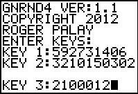
Figure 1	We start the GNRND4 program and use the key values shown in Figure 1. One thing to note here is that based on the values in the first key, the program determines that it requires two additional key values. This difference is continued in Figure 2 where the displayed output consistes of not one but two lists.
Figure 2	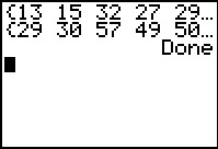GNRND4 displays the first list and pauses to allow the user to scroll across the items of that list. The user presses to signal the calculator
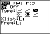
Figure 3	We can plot these pairs of values. We use a coordinate axes system to do this. On the calculator this is called a scatter plot. We press to open the STAT PLOT menu. For the calculator used to generate these images the STAT PLOT menu shows that Plot1 is On but it is set for a histogram, . We need to change this. Press to open the Plot1 settings in Figure 4.
Figure 4	Here is the Plot1 screen before we have changed it. We will move the highlight to the scatter plot icon, . Then we press to change that to .
Figure 5	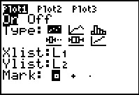Figure 5 shows the changed settings. We note that we did not have to changes the Xlist: setting because our X values are in L1. Likewise, we did not have to changes the Ylist: setting because our Y values are in L2. Now that Plot1 is set, we move to set up the window for the plot.
Figure 6	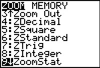Press to open the ZOOM menu and then use the key to move down the the 9th item, ZoomStat. When we select this item, by pressing the key, the calculator will look at the data needed to complete the selected plot. In our current case that will be the values in L1 and L2. Then, based on that data, the calculator will determine what it computes to be the best values for the various WINDOW settings. Having done that, the calculator moves directly to make and show the plot.
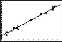
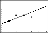
Figure 7	Here is a plot of the X,Y pairs of values. In this case these pairs of values have a strong linear relation. We can see this because the plotted points seem to fall on a straight line. The two questions before us are What is the equation of the line that "best" fits this data? The equation that we find will be the "best" fit, but just how good is that "fit"? The command that will give us all of that information is LinReg(ax+b). However, before we move to that command, we may want to take a slight detour.
Figure 8	Looking ahead, we want to be sure that the calculator being used here has Diagnostics turned ON. Once this has been turned ON for a particualr calculator, it is supposede to stay ON. Therefore, this should be a task that only needs to be done once. Still, it is nice to know how to do it just in case it needs to be done again. If you are sure that your calculator has Diagnostics turned On, then skip to Figure 11. Otherwise follow the steps here. 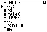We find the command DiagnosticOn in the CATALOG. We open the CATALOG by pressing . Figure 8 shows the start of the CATALOG. The CATALOG lists, in alphabetic order, all of the commands that are available on the calculator. We generally find most of those commands in the various menus. DiagnosticOn is not in a menu. Therefore we need to look for it here in the CATALOG.
Figure 9	We can scroll down to the command. There is a slight help in doing this. If we press , the key tied to the alphabetic character D, then the calculator will jump down to the start of the D entries in the CATALOG. That saves us some scrolling, though we still need to scroll down to the desired command, as shown in Figure 9. Once the command is highlighted, press to paste the command onto the main screen.
Figure 10	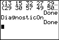Once the command is pasted to the main screen we press to have the calculator perform the command. It responds with Done when it is finished.
Figure 11	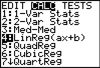Use to open the STAT menu. Use to move to the CALC sub-menu. Use to move the highlight down to 4:LinReg(ax+b), as shown in Figure 11. Press to select that highlighted option and paste it to the main screen.
Figure 12	We now have the right command in place. Given in this fashion, the LinReg(ax+b) command will cause the calculator to compute, from the data in L1 and L2, the coefficient (a) and the constant (b) in the y =ax+b form of the linear equaton that best fits the data in those lists. We press to have the calculator perform the command.
Figure 13	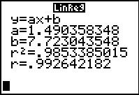The result is shown in Figure 13. Here the calculator reminds us that the form of the linear regression equation is y=ax+b. Then the calculator tells us that the line of best fit will have a=1.490358348 and b=7.723043548. If we were to round these two values to the nearest hundredth, then the linear regression equation could be written as y = 1.49*x + 7.72 Furthermore, the calculator tells us that the correlation coefficient for this data is r=.992642182. This is an extraordinarily high correlation coefficient. Correlation coefficients range from +1 to –1, with high degrees correlation (i.e., having the plotted points be really close to a straight line) being close to +1 and –1. Situations where the plotted points are more spread out, not falling so close to a line, have correlation coefficients closer to zero. We will see this situation on a different web page.

At this point we know the linear regression equation. It would be nice to actually see it on the graph. Fortunately, it is not a huge problem to get the calculator to do this.

One of the primary uses of getting the linear regression equation is to be able to use it, not just graph it. By "use it" we mean that if we are given a value for X then we can put that value into the equation and calculate the expected value of Y. As is usually the case there are many different ways to get the calculator to help us do this. For example, if we were given the value 20 for X then, using the rounded version of the linear regression equation given above, we could type

We could do this same thing with the value 27, calculating

Having two values, an observed and an expected value allows us to form a new value called the residual. We define the residual as

Let us return to the calcualtor to see how to do some of these same things.

Figure 14	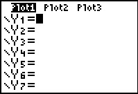The first task is to get the calculator to draw the linear regression equation. To do this we open the Y= window via . The calcualtor is ready for us to type in the right side of the linear regression equation. We might have written it down from Figure 13. We might want to roundoff the coefficient and constant, as we did in the discussion above, or we might want to use the full ten significant digit version that the calculator gave us. Rounding means less typing. There is some question as to where to round, how many digits should we use? If we were toround to the nearest hundredth, then we could enter the equaion here as 1.49*X+7.72, but we are not going to do that. The calculator actually makes it easier to use the equation that it determined rather than to use any rounded version. The calculator can paste the equation that it determined directly into this screen. We just have to find where the calcualtor stored the equation.
Figure 15	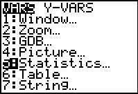We use to open the VARS menu. Then we highlight the fifth item, Statistics... and press .
Figure 16	THis takes us to the VARS Statistics sub-menu. Here we have all sorts of statistics variables that we can recall. However, we want an equation. TO get that we move to the right two times to get tot eh EQ, or equation, sub-menu.
Figure 17	The first item in this sub-menu is RegEQ, our regression equation. We press to select it and to paste it back into our Y= screen.
Figure 18	Here we see that the calculator has pasted the entire original regression equation onto this screen. A closer examination of that equation shows that the calculator actually pasted a 14-digit version of the equation here, not the shorter 10-digit values given in Figure 13. Once the equation is here we can press to return to the graph.
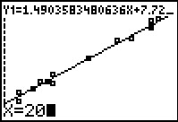
Figure 19	Now, in addition to the plotted points we have the graph of the linear regression line.
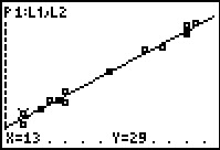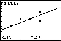
Figure 20	For Figure 20 we have moved into TRACE mode by pressing the key. The calculator starts by "tracing" the plotted points. Note the P1:L1,L2 at the top of the screen. This indicates that the calcualtor is ploting points from Plot1 and that Plot1 is based on L1 and L2. At the bottom of the screen the X=13 and Y=29 indicate the coordinates of the highlighted point. The highlighted point is a bit hard to see here, but it is the point below the arrow in .
Figure 21	Pressing the key takes the trace to the second point in the data. This point is close to the first on the plot, but that is just an accident fo the values in the original list.
Figure 22	Pressing the key takes the trace to the third point in the data. Now we are at the upper right corner of the screen.
Figure 23	Pressing the key takes us from tracing the plotted points to tracing the graph of the equation. Note that the equation being traced is now displayed across the top of the screen. The calculator starts the trace half way across the screen. The bottom of the screen displays the coordinates of the point being highlighted. Somewhat as an accident and somewhat as just poor planning, the highlight on the line is alos on one of the plotted points.
Figure 24	Now, because we are tracing the graph of the line, when we press the key the highlight just moves a little bit to the right along the line. We will have to press the key six times to get to the display in Figure 24. As we move, left or right, the screen updates to show us the X and Y coordinates of the highlighted point. The Y values are the expected value for each of the corresponding X values. We could use this feature to find expected values, but it is a pain to keep moving left and right in such small increments. Also, the choice of X values is a calculator decision. Thus, we can get close to an X value of 24 but we are not going to be right at 24 by moving the highlight left and right like this.
Figure 25	However, when we re in TRACE mode, as we are in Figure 24, we can just type in the desired value of X. Figure 25 is the result o pressing . We will be asking the calcualtor to jump to the point on the line that has an X coordinate of 20. To get the calculator to do this we press .
Figure 26	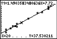Now the trace is at the point X=20 and Y=37.530211, the expected value. We might recall that when we used the rounded linear regression equation our exected value, when X=20 was 37.52. The difference is that the graph here is using all 14 significant digits of the equation and that causes a different, and more accurate, result.
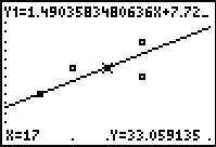
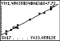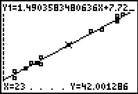
Figure 27	For Figure 27 we have moved the highlight directly to the X value 17 by pressing . Now we see that the associated expected value is 33.059135. We know from the original table that for X=17 the observed value is 33. This makes the associated residual value 33-33.059135 = –0.059135.
Figure 28	We can get a closer look at the data points and the line by changing the WINDOW settigns. We move to the WINDOW menu via . Figure 28 shows the settings as determined by the calculator back in Figure 6 when we used the ZoomStat command.
Figure 29	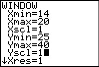Figure 29 shows the modified WINDOW settings. Here we 'have decided to only display X values from 14 to 20 with an Xscl=1. The Y values range from 25 to 40. Once these values are set we can return to the graph via .
Figure 30	The new graph shows only the newly defined area.
Figure 31	We reenter TRACE mode via . The top and bottom of the screen clearly show that we are back in TRACE mode, but our highlighted point, identified at the bottom as X=13 and Y=29 is not highlighted on the screen. This should be expected since we set the X values to range from 14 to 20, leaving X=13 off the screen.
Figure 32	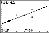Still, we can use the key to move to another point of the data set. As it turns out, the next point, X=15 and Y=30, is indeed on the screen.
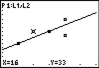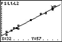
Figure 33	We can continue to look at the points on our plot. In Figure 33 we have moved to the thirteenth point of the plot, X=16 and Y=33.
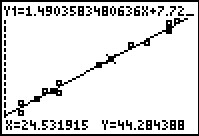
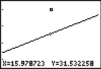
Figure 34	We want to find the residual value at X=16. Therefore, we need to find the value of the linear regression equation when X=16. We use to move from tracing the plotted points to tracing the graph of the equation. The calculator decides to put this trace at X=17.
Figure 35	We prepare to move to X=16 by typing . Then we can get the calcualtor to actually move thre by pressing to take us to Figure 36.
Figure 36	Here the highlight is at X=16 and Y=31.56877. This gives us the expected value. The residual value is the (observed) – (expected), or in this case, 33-31.56877 = 1.43123.
Figure 37	Earlier, in Figures 28 and 29, we brought the focus of the screen into a smaller region than the original settings of the calculator. We can do the same thing, but in a slightly diifferent fashion. To get to Figure 37 we press and then . THis highlights the Zoom In option. Then press to move to Figure 38.
Figure 38	The calculator has a flashing plus sign at the same place where we left the cursor in Figure 36. One might note that we are no longer in TRACE mode here. We can tell that because there is no tracing information at the top of the screen. We can move the flashing plus sign anywhere we want on the screen to pick out the center of our new screen. Once in place, we press and the calculator will "zoom in", adjusting the WINDOW settings so that the selected point in in the center of a new screen and the limits of the new screen will be closer together than they are for the current screen.
Figure 39	Here is the new screen. We have narrowed the view to where we see only the one data point.
Figure 40	Use to return to TRACE mode. Again, the calculator tries to trace the first data point, but it is way off of this screen.
Figure 41	We press to shift the TRACE to the line.
Figure 42	We press to force the calculator to move the the point on the line where X=16. This shows the same expected value that we had before. We do not get a better value by zooming in on the region.
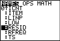
Figure 43	Residual values are so important that the calculator calculates them whenever it does a LinReg(ax+b) command. There is one residual value generated for each of the paired X and Y values. The calcualtor puts these values into a new list that is named RESID. We can find that list by opening the LIST menu, via .
Figure 44	Then we need to sue the key to move down the list until we find the desired RESID name.
Figure 45	We press to select and paste that name onto the main screen. Then we press again to perform that command.
Figure 46	The result is that the items in the list RESID are displayed. Unfortunately, each item is so long that we really only get to see the first item, in this case 1.90229727. We can use the key to scroll over to the right to display more of the elements in the list named RESID.
Figure 47	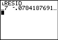Figure 47 shows the start of the second number in RESID. Clearly, this is an inefficient way to look at the residual values.
Figure 48	As an alternative we could go back and once again paste the RESID name onto the screen, but then follow it with as a command to take the values in RESID and copy them to the list L3. At first this does not seem any better because the calculator redisplays the list for us. However, we recall that the StatEditor shows the contents of L1, L2, and L3.
Figure 49	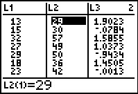Press to get to Figure 49. Here we can see the X values in L1, the Y values in L2, and now the residual values in L3.
Figure 50	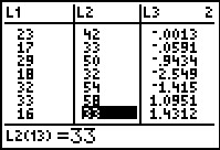If we want to know the residual value associated with the thirteenth data pair, X=16 and Y=33, then we can move down the list to the 13th row and see that the residual value is 1.4312. We could safely exit the StatEditor via the sequence.
Figure 51	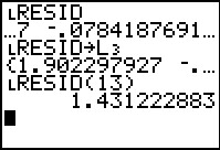Back in the main screen, we see yet another way to look at the residual values. Again, this uses the list of residual values named RESID. We can get a display of any one of the values in that list by pasting the name of the list onto the main screen and tehn following it with the desired index value enclosed in parentheses. Thus the command RESID(13) displays the value in the thirteenth item of the list.