This page is devoted to presenting, in a step by step fashion, the keystrokes and the screen images for obtaining values for a Binomial Distribution on a TI-83 (TI-83 Plus, or TI-84 Plus) calculator.

Recall that in a binomial distribution there are only two possible outcomes to an experiment (an event), one of which we term a success while the other is termed a failure. On any one trial of the experiment the probability of a success is denoted as `p`. Therefore, on any one trial of the experiment the probability of a failure must be `1-p`. We use the variable `n` to denote the number of trial that we want to run. For `n` trials the probability that we will get `x` successes is given as

• the mean of `X` is `mu_X = np`
• the variance of `X` is `sigma_X^2 = np(1-p)`
• the standard deviation of `X` is `sigma_X = sqrt( np(1-p) )`

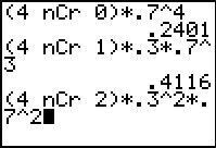
Figure 1	The case we will examine here is to have `n` trials with a probability of success `p=0.3`. Using the equation `P(x) = quad_nC_xp^x(1-p)^(n-x)` we could realy compute the probabilty of 0 successes. The equation becomes `P(0) = quad_4C_0*.7^4`. We construct that on the main screen, shown in Figure 1. In that Figure we also see the value of `P(0)=.2401`, the expression for `P(1) = quad_4C_1*.3*.7^3`, the value of `P(1)=.4116` and the expression for `P(2) = quad_4C_2*.3^2*.7^2`.
Figure 1a	We continue in Figure 1a with the value of `P(2)=.2646`, the expression for `P(3) = quad_4C_3*.3^3*.7^1`, and the value of `P(3)=.0756`.
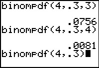
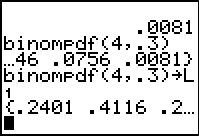
Figure 1b	We conclude all the possible results from `4` trials with the expression for `P(4) = quad_4C_4*.3^4` and the value of `P(4)=.0081`. Seeing that we can do this is nice, but it would be so much more convenient for the calculator to help us on this. To that end the calculator is designed to give us certain probability distributions, one of which is the binomial distribution.
Figure 1c	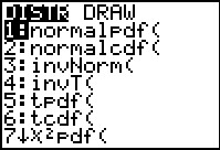To get to the image in Figure 1c we press . This takes us to the DIST (distribution) menu. The operation that we want, binompdf(, is not shown here. We need to move down the menu to find it. The pdf in binompdf( stands for probability distribution function.
Figure 2	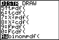In FIgue 2 we have moved down the menu to locate and highlight binompdf(. We perss to select and paste that item.
Figure 3	Figure 3 shows the pasted text binompdf(. That command will compute the binomial probability for a case where, for we have a given number of trials and a given probability of success, we want the probability of a specific number of successes. To do this we need to tell the calculator all three of those values: number of trials probability of a success on a single trial specific number of successes for which we want this computed Our problem is to remember the sequence in whch we are to supply these values.
Figure 4	The binompdf( command wants the values in exactly the order that we have listed them above. In Figure 4 we have asked for the binomial distribution probability that in 4 trials with a probability of a single success being 0.3 we find 0 successes. Press to have the calculator perform the command.
Figure 5	The result, shown in Figure 5, is .2401, exactly what we computed in Figure 1. We have gone further in Figure 5 by recalling the previous command via and then using the cursor keys to move back to the command and to change the specification of the desired number of successes to 1. Again, we perform the command via and move to Figure 6
Figure 6	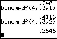Here we see that the `P(1)=.4116`, that we have again recalled the command, modified it to ask for the probability of exactly 2 successes, and found that `P(2)=.2646`.
Figure 7	In Figure 7 we complete the study by finding the two remaining probabilities. The values have not changed from our earlier calcualtions but the process is a bit easier.
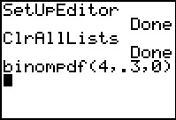
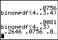
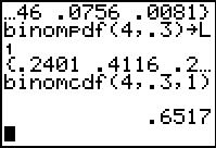
Figure 8	The binompdf( command has one other useful feature, namely, if we omit the final field then the command computes the probabilities for each of the possible values for that field putting the answer in the form of a list of values. At the bottom of Figure 8 we have formed and performed the command binompdf(4,.3).
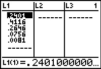
Figure 9	We perform the command via . The calcualtor displays the first portion of the answer, the list of values for P(0), P(1), and the start of P(2).
Figure 10	We can scroll across this to see more of the values.
Figure 11	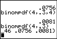In Figure 11 we have finished scrolling and we now see the last of the values.
Figure 12	Because the binompdf(4,.3) command produces a list we can assign that list to a list in the calculator. For Figure 12 we have recalled the command and appended the action. Then we performed the command via. The result seems to be the same as before, namely a display of the computed values.
Figure 13	However, if we move to the StatEditor we see the entire list of values has been stored in L1. One major word of caution here. Note that index 1 of the list, that is L1(1) holds the value for P(0), not P(1). To find P(1) we need to look at index 2, namely, L1(2). Now that we have the values in L1 it would be easy for us to create the cumulative sum of those values in L2. We could just move to the LIST menu, then to the OPS sub-menu, select the cumsum( option and formulate and execute the command cumsum(L1)L2.
Figure 14	Rather than do that, the calculator provides another command, binomcdf(, that computes the cumulative probability distribution for specified values. In fact, the values are in the same order as we hade in the earlier binompdf( command. The only difference is that for the binomcdf( command the interpretation of the result is changed giving the sum of the probabilities of having the number of successes in n trials with 0 up to and including the specified number of successes. We use to return to the DIST menu. Then we move down th menu to find binomcdf(.
Figure 15	Having found and highlighted the option, press to paste it onto the main screen.
Figure 16	In Figure 16 we have completed the command by indicating that we are looking at 4 trials where the probability of a single success is 0.3, and we want the probability that the number of successes in those four trials is less than or equal to 1. The result, .6517 is just what we would expect since we know, from Figure 13 that we expect the anser to be the sum .2401+.4116.
Figure 17	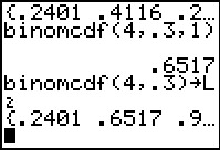binomcdf( works the way binompdf( did in that if we omit the final value then the result is a list of values, one for each of the possible number of successes. In Figure 17 we have made such a command and put the result into L2. The start of the resulting list is shown on the screen.
Figure 18	We return to the StatEditor and we see the new values in L2. We could use these to solve a number of different kinds of problems, but why use the table when the binompdf( and binomcdf( commands recompute the values any time we want them?

Binomial distribution probabilities lend themselves to just six kinds of problems. We will look at these, but we will pose them in the setting of having 17 trials with a 0.385 probability of success. Here are the six types of questions, with specific values for illustration:

1. What is the probability that we get exactly 10 successes?
2. What is the probability that we get 10 or fewer successes? Note that we could rephrase this as getting no more than 10 successes. A slight variation on this is to ask for the proability of getting fewer than 10 successes, but that is the same as asking for the probability of getting 9 or fewer successes.
3. What is the probability of that we get 10 or more successes? Note that we could rephrase this as getting no fewer than 10 successes. A slight variation on this is to ask for the probability of getting more than 10 successes, but this is the same as asking for the probability of getting 11 or more successes.
4. What is the probability of getting between 4 and 10 successes, inclusive of 4 and 10? A slight variation on this is to ask for the probability of getting strictly between 4 and 10 successes, but this is the same as asking for the probability of getting between 5 and 9 successes inclusive of 5 and 9.
5. What is the probabilty of getting 5, 8, or 11 successes? The point here is that the values chosen are not consecutive so that we cannot phrase this as a type 4 problem.
6. What is the probability of not getting 10 successes? There are many variations of this. The important point is that this type of question asks for the probability of something not happening.

Create the L1 and L2 lists
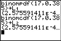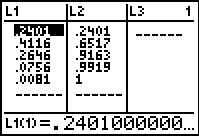
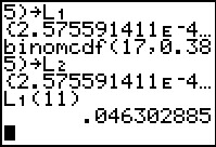
Figure 19	First we will generate the two lists, the proability valeus and the cumulative probability values, in L1 and L2, respectively. We note here that the P(0) is given as 2.575591411E–4, meaning 2.575591411*10–4.. To express this number without the power of 10 we just need to move the decimal point 4 places to the left to get 0.0002575591411.
Use the StatEditor to inspect the values in those lists.
Figure 20	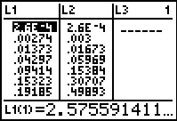Then we move to the StatEditor to inspect those values. Unfortunately, we can only see 7 values for each list at a time in the editor. Note that the value of L1(1), which holds P(0) is given as 2.6E–4, meaning 2.6**10–4. To express this without using the power of 10 we just move the decimal point four places to the left to get 0.00026. We also note that the values in the table portion of the display have been rounded to use only 5 characters (6 including the decimal point). We can still see the full value for a specific item by highlighting that item in the table. It is also important to remember that the index for items in the list corresponds to having one fewer than the index number of successes. Thus, the seventh item in L1, namely .19185, corresponds to P(6).
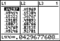
Figure 21	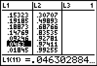In Figure 21 we have moved down the list and then back up one iotem so that the highlight is on L1(11) which corresponds to P(10).
Figure 22	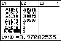Moving down to the bottom of the list, the display is now at L1(18) which corresponds to P(17), showing a value there of 9E–8, meaning 9*10–8 which we would expand, by moving the decimal 8 places to the left, as 0.00000009. Of course, seeing the more accurate 8.97082535... at the bottom of the screen, we realize that the 9 shown in the table value 9E–8, is just the rounded version of 8.97082535.... We have no way on this screen to see the rest of 8.97082535.... Once we are back to the main screen we could just type L1(18) to see the rest of this entry. It would appear as 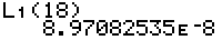. Thus, the more accurate expansion would be 0.0000000897082535, not that we would ever need such accuracy in a real problem.
Figure 23	Q1:  To answer "What is the probability that we get exactly 10 successes?" we just need to move back to see the value in L1(11). Therefore, the answer is 0.0463. Q2:  To answer "What is the probability that we get 10 or fewer successes? we read across to the value in L2(11). Therefore, the answer is 0.97411. Q3:  To answer "What is the probability of that we get 10 or more successes?" we need to realize that the answer will be 1-P(x≤9), and that the value of P(x≤9) is at index 10 of L2. Therefore, the answer is 1 – 0.92781 or 0.07219.
Figure 24	Q4:  To answer "What is the probability of getting between 4 and 10 successes, inclusive of 4 and 10?" we need to realize that the answer will be P(x≤10)-P(x≤3). We saw above that P(x≤10) is 0.97411. We move back up the table to find the value of P(x≤3) is at index 4 of L2, namely, 0.05969. Therefore, the answer is 0.97411 – 0.05969 or 0.91442. Q5:  To answer "What is the probabilty of getting 5, 8, or 11 successes?" we need to realize that the answer will be the sum of the probabilities or getting exactly 5, exactly 8, and exactly 11 successes. We have seen all of these in the various screens in the L1 column. The value of P(x=5) is at index 6 of L1, namely 0.15323. The value of P(x=8) is at index 9 of L1, namely 0.14769. The value of P(x=11) is at index 12 of L1, namely 0.01845 (see Figure 21). Therefore, the answer is 0.15323+0.14769+0.01845 or 0.31937. Q6:  To answer "What is the probability of not getting 10 successes?" we need to realize that the answer will be 1-P(x=10), and that the value of P(x=9) is at index 11 of L2. Therefore, the answer is 1 – 0.0463 or 0.9537. (This is the same technique that we used in question type 3. However, this is a more general statement. To get the probability of not getting some value, or values, take 1 minus the probability of getting that value (or those values).
Use the direct reference to values in the lists.
Figure 25	We will do all of the problems again, this time using direct references to the values that we stored in L1 and L2 back in Figure 19. Q1:  To answer "What is the probability that we get exactly 10 successes?" we want P(x=10) which is stored in L1(11). The answer is 0.046302885.
Figure 26	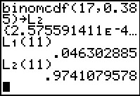Q2:  To answer "What is the probability that we get 10 or fewer successes?" we want P(x≤10) which is stored in L2(11). The answer is 0.9741079578.
Figure 27	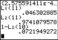Q3:  To answer "What is the probability of that we get 10 or more successes?" we need to realize that the answer will be 1-P(x≤9), and that the value of P(x≤9) is at index 10 of L2. Therefore, we get the answer from 1–L2(10) which gives 0.0721949272.
Figure 28	Q4:  To answer "What is the probability of getting between 4 and 10 successes, inclusive of 4 and 10?" we need to realize that the answer will be P(x≤10)-P(x≤3). The value of P(x≤10) is at L2(11). The value of P(x≤3) is at L2(4). Therefore, we get the answer from L2(11)–L2(4) which gives 0.9144142597.
Figure 29	Q5:  To answer "What is the probabilty of getting 5, 8, or 11 successes?" we need to realize that the answer will be the sum of the probabilities or getting exactly 5, exactly 8, and exactly 11 successes. We have all of these in L1(6), L1(9), and L1(12), respectively. Therefore, we get the answer from L1(6)+L1(9)+L1(12) which gives 0.31936849.
Figure 30	Q6:  To answer "What is the probability of not getting 10 successes?" we need to realize that the answer will be 1-P(x=10), and that the value of P(x=9) is at index 11 of L2. Therefore, we get the answer from 1–L1(11) which gives 0.953697115. (This is the same technique that we used in question type 3. However, this is a more general statement. To get the probability of not getting some value, or values, take 1 minus the probability of getting that value (or those values).
Just use binompdf( and binomcdf( directly.
Figure 31	We will do all of the problems again, this time using direct references to the binompdf( and binomcdf( commands. For thise we did not even need to do the steps in Figure 19. Q1:  To answer "What is the probability that we get exactly 10 successes?" we want the binompdf(17,0.385,10) command. It produces 0.046302885.
Figure 32	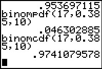Q2:  To answer "What is the probability that we get 10 or fewer successes?" we want the binomcdf(17,0.385,10) command. It produces 0.9741079578.
Figure 33	Q3:  To answer "What is the probability of that we get 10 or more successes?" we need to realize that the answer will be 1-P(x≤9). The command 1- binomcdf(17,0.385,9) produces 0.0721949272.
Figure 34	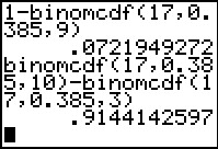Q4:  To answer "What is the probability of getting between 4 and 10 successes, inclusive of 4 and 10?" we need to realize that the answer will be P(x≤10)-P(x≤3). The command binomcdf(17,0.385,10)-binomcdf(17,0.385,3) produces 0.9144142597.
Figure 35	Q5:  To answer "What is the probabilty of getting 5, 8, or 11 successes?" we need to realize that the answer will be the sum of the probabilities or getting exactly 5, exactly 8, and exactly 11 successes. The command binompdf(17,0.385,5)+binompdf(17,0.385,8)+binompdf(17,0.385,11) produces 0.31936849.
Figure 36	Q6:  To answer "What is the probability of not getting 10 successes?" we need to realize that the answer will be 1-P(x=10). The command 1-binompdf(17,0.385,10) produces 0.953697115. (This is the same technique that we used in question type 3. However, this is a more general statement. To get the probability of not getting some value, or values, take 1 minus the probability of getting that value (or those values).