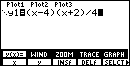
The TI-86 allows us to graph parametric equations. This
page demonstrates two examples of graphing parametric equations.
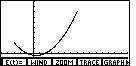
However, before we even start that process, we will us the first six Figures to quickly
review the steps used in graphing functions. We will obtain the graph of the
function
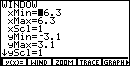
So much for the review of graphing functions. Now we want to look at the
steps needed to graph parametric equations. We will use the following as
our example:
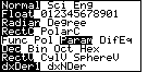
In order to have the TI-86 graph parametric equations we need to shift it into
parametric mode.
Figure 7
| We return to the MODE screen by pressing
the   keys. THen
we move down to the fifth line by using the keys. THen
we move down to the fifth line by using the  key four times. Next we move the blinking cursor to the right by pressing
the
key four times. Next we move the blinking cursor to the right by pressing
the  key twice. And, finally, we actually select
Parametric mode by pressing the key twice. And, finally, we actually select
Parametric mode by pressing the  key.
The result is as shown
in Figure 7. key.
The result is as shown
in Figure 7. |
Figure 8
| We use the  key to open the GRAPH
menu shown in Figure 8.
Note that the first menu item has been changed. Where we used to
find the y(x)= option, we now find the E(t)= option. key to open the GRAPH
menu shown in Figure 8.
Note that the first menu item has been changed. Where we used to
find the y(x)= option, we now find the E(t)= option. |
Figure 9
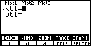
| Pressing  to select that E(t)= option,
the calculator displays the screen that prompts us for the two parametric
equations. The first equation needs to give x as a function of t, while
the second equation needs to give y as a function of t. to select that E(t)= option,
the calculator displays the screen that prompts us for the two parametric
equations. The first equation needs to give x as a function of t, while
the second equation needs to give y as a function of t. |
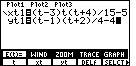
Figure 10
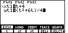
| In Figure 10 we have entered the parametric equations for our problem.
Note that we generate the t in the equations by using the
key to select the t from the sub-menu. |
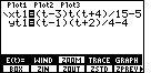
Figure 11
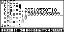
| Next, we will check out the settings for the
WINDow screen. We press  to select WIND from the top menu of Figure 10. This produces
Figure 11, where the blinking cursor is covering the value 0.
to select WIND from the top menu of Figure 10. This produces
Figure 11, where the blinking cursor is covering the value 0.
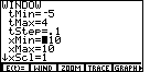
This screen, the WINDOW screen for parametric mode, has three new values in it,
tMin, tMax, and tStep. These settings will be used to
create the values of t that will be used to plot our equations.
You might notice that although tMax is not a nice even value,
it is not just a random value. Rather, tMax is twice the value of
 . tStep is set so that there are
49 values of t to be plotted, from tMin through tMax. . tStep is set so that there are
49 values of t to be plotted, from tMin through tMax.
|
Figure 12
| Figure 11 displayed the first six values in the
parametric equation WINDOW screen. We can
use the key to scroll
down so that we can see the remaining 3 values on that screen. |
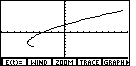
Figure 13
| We press  to actually graph the equations.
The TI-86 will generate each of the 49 values of t from tMin through
tMax. For each value of t, the calculator determines the appropriate
value of x and y from the parametric equations. Then, the calcualtor
graphs that (x,y) point on the screen. to actually graph the equations.
The TI-86 will generate each of the 49 values of t from tMin through
tMax. For each value of t, the calculator determines the appropriate
value of x and y from the parametric equations. Then, the calcualtor
graphs that (x,y) point on the screen.
When t is 0 we will get x=4 and y=0. Therefore, the first
point that is graphed is the point (4,0). |
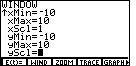
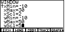
Figure 14
| We can see from Figure 13 that we need to change the
values that will be assigned to t. We press the
key to return tot he WINDOW screen.
Then, in Figure 14, we have changed the values of tMin, tMax, and
tStep, so that t will vary from – 10 to 10 in steps of
one tenth. |
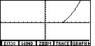
Figure 15
| We press to initiate a new graph, based on the new
values for t. The new graph appears in Figure 15. |
Figure 16
| Pressing  shifts the calculator into TRACE mode. Note that the calculator displays the
values of t, x, and y at the bottom of the screen.
We start at the lowest value of t, that is at tMin.
shifts the calculator into TRACE mode. Note that the calculator displays the
values of t, x, and y at the bottom of the screen.
We start at the lowest value of t, that is at tMin.
|
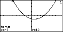
Figure 17
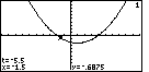
| The calcualtor allows us to trace the graph by changing the value
of t. Each time we move the cursor left or right, the
calculator changes t according to the value in tStep
and within the limits of tMin and tMax.
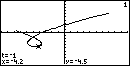
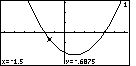
For example, in Figure 17, we have used the
key to move the cursor to the right
until t has the value – 5.5, which means that
x=– 1.5 and y=– 0.6875. |
Figure 18
| The graph in Figure 17 pretty much filled the
calculator image. Let us return to the
WINDOW settings and make some changes to enlarge the range
of the values that we will display. Figure 17 was in TRACE mode.
We press
 to leave TRACE mode and restore
the menu. Then press to select the
WIND option. This will display the various WINDOW settings.
For Figure 18 we have used the
key to move down that list of values,
changing the xMax, xScl, yMax, and yScl values as shown. to leave TRACE mode and restore
the menu. Then press to select the
WIND option. This will display the various WINDOW settings.
For Figure 18 we have used the
key to move down that list of values,
changing the xMax, xScl, yMax, and yScl values as shown. |
Figure 19
| We press
to generate a new graph, based on the changed WINDOW settings.
That graph, shown in Figure 19 demonstrates the limits on the graph
imposed by having t take on values between – 10
and 10. |
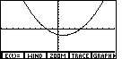
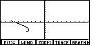
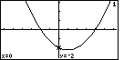
The function graph in Figure 6 looks remarkabley like the parametric
equation graph of Figure 17. In fact, these are the same relations.
If westart with our function
That first example allowed us to convert a function to parametric equations.
However, this does not demonstrate the power and flexibility of
parametric equations. To do this, consider the parametric equations
Figure 20
| We return to the E(t)= screen
by pressing the key.
Then we enter the equations to replace the ones that
were using earlier. Figure 20 reflects the new equations.
|
Figure 21
| Before we graph these equations
we press  to open the ZOOM sub-menu. This is shown in Figure 21.
 |
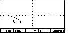
Figure 22
| We press to select the
ZSTD option from the sub-menu in Figure 21. That option
will set the standard values into the various WINDOW settings,
and it will produce the graph of the parametric equations.
That graph is shown in Figure 22. We immediately note that the graph in Figure 22
is NOT a function. It fails the vertical line test.
In addition, given the standard settings, we are not sure just
what the rest of the graph should look like. We need to go
back and modify those settings.
|
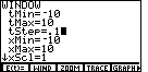
Figure 23

| We return to the WINDOW screen by pressing
the key. Figure 23 shows the
standard settings for parametric equations. |
Figure 24
| Figure 24 shows the WINDOW settings after we
have made some modifications. We will let t run from
– 5 to 4 in steps of 0.1.
|
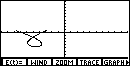
Figure 25
| To start Figure 25 we press the
key. Doing so will actually
generate Figure 27. However, in Figure 25 we have caught the
graph in progress. In this fashion we can see that the
graph starts at about (– 7.7,0.5)
and it sweeps to the right and down, only to turn back to the left
at about x=– 3.5. |
Figure 26
| Figure 26 represents a further step in the graph as it moves to completion
in Figure 27. Note that the horizontal motion has changed back to
moving toward the right. And, we are no longer seeing
the graph go down; now it is moving up. |
Figure 27
| Figure 27 has the complete graph. Complete, that is, within the limits
that we imposed on t back in Figure 24.
If we change those values, we will change the graph. |
Figure 28
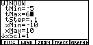
| In Figure 28 we have returned to the WINDOW settings by pressing
. In addition, we have altered the setting for
tMax to be 6. |
Figure 29
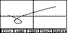
| Press to draw a new graph, shown in Figure 29.
|
Figure 30
| As before, we press the
key to move into TRACE mode. Note that the calculator
displays the appropriate values of t, x, and y. |
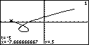
Figure 31
| Now that we are in TRACE mode, we press
the key to move the trace pointer to the next
value of t.
In Figure 31 we have pressed that key about 20 times to move the pointer
to near the right edge of the loop. |
Figure 32
| If we continue to press the
key, the trace indicator continues to follow the graph, just as
we saw it being drawn back in Figures 25 through 27. Note that t
continues to increase, even though x and y
may be increasing or decreasing. |
Figure 33
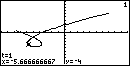
| Figure 33 merely continues the demonstration of the
TRACE mode, using the key
to move the pointer to the next value of t. |
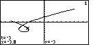
 key 15 times we move the trace indicator to the position shown in
Figure 6. At that point x is – 1.5 and y is
– 0.6875.
key 15 times we move the trace indicator to the position shown in
Figure 6. At that point x is – 1.5 and y is
– 0.6875.