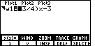
| Example 14: Graph y |
Example 15: Graph y1 = 5x + 2 and y2 = x – 6 and shade the region where y1 |
 |
 |
| Example 14: Graph y |
Example 15: Graph y1 = 5x + 2 and y2 = x – 6 and shade the region where y1 |
| |
|
|
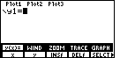
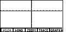
We start by moving to the graph menu via the
 key and then selecting the y(x)= option via
the key and then selecting the y(x)= option via
the  key. This produces Figure 1. key. This produces Figure 1.
|
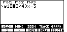
| In Figure 2 we have entered the line we wish to graph via the keys
 
 
 and .
Note that this is an equality. We expect that the graph will be a line. and .
Note that this is an equality. We expect that the graph will be a line.
|
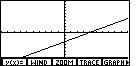
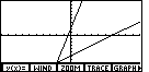
| We leave Figure 2 and move to Figure 3 by pressing
 and and  . The resulting graph,
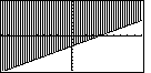
done with the Zoom Standard settings, is the expected line. However, we wanted to
prduce the graph in the book. It has "shaded" the portion of the graph above the line. . The resulting graph,
done with the Zoom Standard settings, is the expected line. However, we wanted to
prduce the graph in the book. It has "shaded" the portion of the graph above the line.
|
| We return to the y(x)= screen via the
key. Note that the resulting sub-menu has
options not currently displayed. This is indicated by the small
arrow at the extreme right of the menu.
|
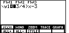
| We press
 to see the additional options. These are shown
in Figure 5. The third option, STYLE, is the one that we will be using.
That option allows us to change the style for the graph. to see the additional options. These are shown
in Figure 5. The third option, STYLE, is the one that we will be using.
That option allows us to change the style for the graph.
|

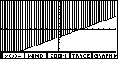
| Figure 6 is the result of pressing
 . The only visible
change from Figure 5 to FIgure 6 is the alteration of the "style indicator", the
small icon to the left of our function definition. In Figure 6 that
icon suggests shading above the graph of the function. . The only visible
change from Figure 5 to FIgure 6 is the alteration of the "style indicator", the
small icon to the left of our function definition. In Figure 6 that
icon suggests shading above the graph of the function.
|
| We return to redraw the graph by pressing
to select the
GRAPH option from the upper menu of Figure 6. This Figure does indeed
look like the one inthe textbook, except that we have the menu displayed
in Figure 7.
|
|
| We can hide that menu, from Figure 7, by
pressing the |
We have produced the graph for Example 14 from the textbook. Example 15 requires us to shade an area between two functions. We do not do this with the normal graphing commands. Rather, the TI-85 and TI-86 have a special command called Shade to do this task. In preparation for using the Shade command we will clear off the graph generated above.
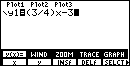
| In Figure 8 we had hidden the menu. We press
 to resore that menu.
Then we press to select the y(x)= option
and to return us to the screen shown in Figure 9. to resore that menu.
Then we press to select the y(x)= option
and to return us to the screen shown in Figure 9.
|

| Pressing the |

| Our next goal will be to start the
Shade command. We can find that command on a sub-menu under
the Graph menu. However, we want to get out of the
y(x)= screen. Therefore, we press
to close the sub-menu, and then to close the
main menu. That way we can press
to re-open the Graph menu,
but to do so outside of the y(x)= screen. Finally,
we generate Figure 11 by pressing the
key to see additional menu options.
|
| We select the DRAW option by pressing
the  key. This will open the sub-menu
shown in Figure 12. We note that Shade is the first option
in that sub-menu. key. This will open the sub-menu
shown in Figure 12. We note that Shade is the first option
in that sub-menu. |
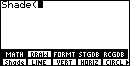
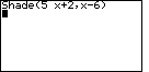
| We press to select the
Shade command. The calculator responds by pasting
Shade( onto the screen. |
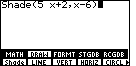
| We complete the basic form of the Shade command by giving the
expression for the lower function (pressing
 
  ), then generating a
comma via ), then generating a
comma via
 , then giving the expression for the
upper function (pressing , then giving the expression for the
upper function (pressing
 , and ending the
command with a closing right parenthesis, , and ending the
command with a closing right parenthesis,
 . The command indicates that the calculator should
DRAW the two functions and it should fill in any part of the screen that is above the
"lower" function and below the "upper" function. . The command indicates that the calculator should
DRAW the two functions and it should fill in any part of the screen that is above the
"lower" function and below the "upper" function.
|
| We constructed the Shade command in Figure 14. Now, press
 to perform the command.
The calculator responds with Figure 15. Actually,
as the calculator draws the graph, it is clear that the desired shading has been done.
However, once the menu of Figure 15 has been displayed, we can no longer see the
shaded portion of the graph. to perform the command.
The calculator responds with Figure 15. Actually,
as the calculator draws the graph, it is clear that the desired shading has been done.
However, once the menu of Figure 15 has been displayed, we can no longer see the
shaded portion of the graph. |
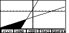
| As before, we can press Still, this is not quite the display that we want to produce. We need to change the WINDOW settings so that we can squeeze more of the range values onto the screen. |
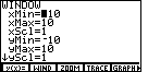
| We press
to restore the menu, and then to open the
WINDOW screen. As expected, the settings shown in Figure 17 are those
of the Zoom Standard feature. |
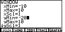
| We will aler those settings by changing the
minimum y value. We press  to move the
highlight down to the yMin line. Then we press
to move the
highlight down to the yMin line. Then we press 
 to enter the new value. to enter the new value.
|
| We return to the graphics screen by pressing
the key. This has been done to generate
Figure 19. But our shaded gaph has disappeared. It has gone away because we
changed the WINDOW settigs and because it was DRAWn, not graphed, by
the Shade command. |
| We leave the graphics display of Figure 19 by
pressing the key. This returns us to the
normal screen we we see the Shade command as our last command. |
|
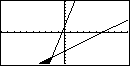
| We need only press to
execute that lst command again and therefore to draw the
lines and shaded region shown in Figure 21.
This is more similar to the graph in the textbook.
We need only hide the menu to have our image be almost identical to that graph.
|
PRECALCULUS: College Algebra and Trigonometry
© 2000 Dennis Bila, James Egan, Roger Palay