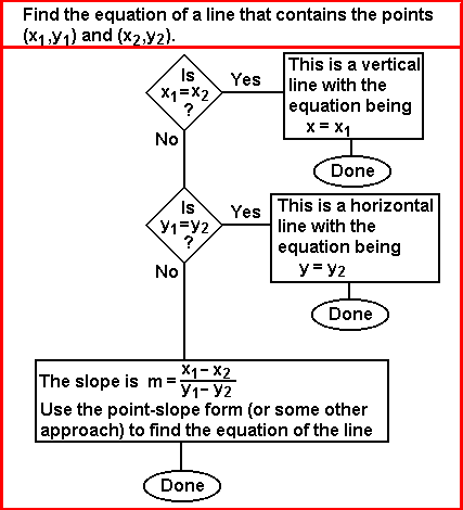

Such an algorithm can be programmed into the calculator. The SLOPE program on the TI-86 (or on the TI-85) implements such an algorithm. Note that the SLOPE program uses the TOSTR program in order to generate nice looking output. The TI-86 version of the SLOPE program is available as slope.86p and the TI-85 version of the SLOPE program is available as slope.85p. The versions of TOSTR, presented in the 208604.htm page, are available as tostr.86p and tostr.85p.

|
We can start by pressing the  key to open the PRGM menu.
Then we press the key to open the PRGM menu.
Then we press the  key to open the NAMES
sub-menu. The calculator used to generate Figure 1 holds a large
number of programs. The program names (or abbreviations of those names)
are displayed in alphabetic order. We will use the key to open the NAMES
sub-menu. The calculator used to generate Figure 1 holds a large
number of programs. The program names (or abbreviations of those names)
are displayed in alphabetic order. We will use the
 key to shift the sub-menu display untilt he SLOPE program is
visible. key to shift the sub-menu display untilt he SLOPE program is
visible.
|

| Figure 2 reflects the condition of having found the
SLOPE program in the sub-menu, and of pressing the
 key to select that program and to paste its name onto the screen. key to select that program and to paste its name onto the screen.
We can execute the command and start running the program by
pressing the |

| In Figure 3, the program has started. The program clears the screen and
displays "Get Slope, etc." on the top line, followed by a
prompt for the value of "x1" on the second line.
We are looking for the solution to "Find the equation of the line containing the points
  for x1.
The program accepts that value and continues by asking for the value
for y1. for x1.
The program accepts that value and continues by asking for the value
for y1.
  assigns 7 to y1.
This is followed by assigns 7 to y1.
This is followed by  
 to give x2 the value 10,
and to give x2 the value 10,
and  to leave the screen as it appears
in Figure 3. to leave the screen as it appears
in Figure 3.
|

| We moved from Figure 3 to Figure 4 by
pressing the  key, and then waiting for the
calculator to do its work. In response the calculator computes the slope,
given as – 1 in Figure 4, and it then continues to generate the
slope-intercept and the standard form of the resulting equation. key, and then waiting for the
calculator to do its work. In response the calculator computes the slope,
given as – 1 in Figure 4, and it then continues to generate the
slope-intercept and the standard form of the resulting equation.
At that point the program is in a "paused" condition, waiting for us to press the ENTER key to continue. The "moving" line of dots in the upper right corner of the screen indicate that "paused" condition. We press |

| The program has started over, from the beginning. The screen has been cleared,
the heading has been rewritten, and the program prompts for values of the coordinates of our
two points. In this case we are solving the problem:
"Find the equation of the line containing the points
 to accept the final value and move to Figure 6. to accept the final value and move to Figure 6.
|

| The calculator has determined the slope, the slope-intercept form
of the solution, and the standard form of the solution.
Please note that the SLOPE program produces a standard form version of the equation that does not require the leading coefficient to be non-negative. |

| Figure 7 represents the data input for yet another example:
"Find the equation of the line containing the points
|

| The calculator has determined the slope between the two points to be
|

| Figure 9 represents the data input for yet another example:
"Find the equation of the line containing the points
|

|
The calculator has determined the slope between the two points to be
|

| Figure 11 represents the data input for yet another example:
"Find the equation of the line containing the points
|

| The SLOPE program correctly identifies the equation as the constant function,
with the solution equation being y=9.
Note that we could write this as y=0x+9 to produce the strict slope intercept form.
In addition we could write this as |

| Figure 13 represents the data input for yet another example:
"Find the equation of the line containing the points
|

| The SLOPE program correctly identifies the equation as a vertical line
with the solution equation being x=6.
Note that we could write this as |

| If we want to stop the program we need to break out of it. We can press the
 key to break out of the program. The result is shown in Figure 15.
There are only two options. Either we can GOTO or QUIT. We want to
QUIT, so we press the key to break out of the program. The result is shown in Figure 15.
There are only two options. Either we can GOTO or QUIT. We want to
QUIT, so we press the  key to move to Figure 16. key to move to Figure 16.
|

| Figure 16 looks remarkably similar to Figure 14. However, in Figure 14 the calculator was in a "paused" condition. In Figure 16 we are out of the program and ready to do anything that we want to do. |
The SLOPE program is designed to generate an equation if we are given the coordinates of two points on the line. How can we use the SLOPE program to solve problems such as
| Find the equation of the line that has slope=4/7 and that contains the point (9,6). |
| m = | 4 | = | change in y |
| 7 | change in x |

| Figure 17 shows that the program has been restarted.
Having broken out of the program in Figures 15 and 16, we only needed to
press the  key to re-issue the
the last command, namely SLOPE, and therefore restart the program.
In Figure 17 we have entered the two points derived from the discussion above.
We can press key to re-issue the
the last command, namely SLOPE, and therefore restart the program.
In Figure 17 we have entered the two points derived from the discussion above.
We can press  to accept the value for y2 and
to move to Figure 18. to accept the value for y2 and
to move to Figure 18. | |||||||||

| The first thing to notice in Figure 18 is that the slope has been computed to be exactly the value given in the problem statement. This is verification that we have correctly computed the coordinates of the second point. Then we can look at the slope-intercept and standard forms for the desired equation. | |||||||||

| The next problem to consider is
| |||||||||

| Figure 20 confirms the second point by calculating the expected slope. Then, the SLOPE program produces the slope-intercept and the standard forms of the desired equations. | |||||||||

| The next problem to consider is
| |||||||||

| Figure 20 confirms the second point by calculating the expected slope. Then, the SLOPE program produces the slope-intercept and the standard forms of the desired equations. |
PRECALCULUS: College Algebra and Trigonometry
© 2000 Dennis Bila, James Egan, Roger Palay