The graphical solution to Example 14 Chapter 1 Section 2 of the text
is not quite as simple to construct as one might hope. That example
uses the problem
Figure 1

|
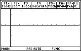
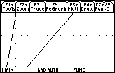
Figure 1 shows the result of pressing the 
 keys
on a TI-89 calculator. The actual output depends on the previous state of the
calculator. In this example, it would appear that no functions have been defined and
that the window settings are not at all standard. keys
on a TI-89 calculator. The actual output depends on the previous state of the
calculator. In this example, it would appear that no functions have been defined and
that the window settings are not at all standard.
|
Figure 2

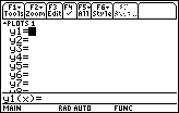
| Press the 
 keys
to see the "y(x)=" list. On this calculator that list is empty. The
calculator is ready to receive the first function definition. keys
to see the "y(x)=" list. On this calculator that list is empty. The
calculator is ready to receive the first function definition. |
Figure 3

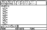
| To produce Figure 3 we have pressed the
 
 and and  keys
to create the first function, which appears on the data entry
line at the bottom of the screen. keys
to create the first function, which appears on the data entry
line at the bottom of the screen.
|
Figure 4

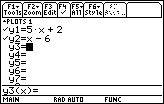
| Then we press the
 key to move to complete
the entry of the first function. This places the first function in the "y1=" line
of the display. In addition, the calculator is now ready for the second function.
That function is created by the key to move to complete
the entry of the first function. This places the first function in the "y1=" line
of the display. In addition, the calculator is now ready for the second function.
That function is created by the
  and and
 keys.
Again, we press the keys.
Again, we press the  key
to accept the second function. It, too, is displayed at the top, in the
"y2=" line. key
to accept the second function. It, too, is displayed at the top, in the
"y2=" line. |
Figure 5

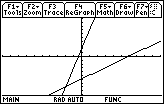
| Having entered the functions in Figures 3 and 4, we press
  to select the GRAPH command. The result is shown in Figure 5.
We can see the graphs of the two straight lines in Figure 5, but this graph does not appear
as does the graph in the text. Part of that difference is due to the
greater screen resolution available on the TI-89. However,
the fact that the point of intersection for the two lines is not visible
and the fact that the lines seem to be at different angles than the
lines in the textbook graph are related to the WINDOW settings,
not to the finer resolution of the TI-89. We will look at the WINDOW settings to see
the current values and to change those values if need be.
|
Figure 6

| To open the WINDOW menu we press the

 key.
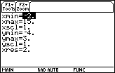
The result is shown in Figure 6. Clearly these are not the
values that we want
to be using. Rather than type all new values, let us use the ZOOM menu
to change the WINDOW settings. To do this,
press the key.
The result is shown in Figure 6. Clearly these are not the
values that we want
to be using. Rather than type all new values, let us use the ZOOM menu
to change the WINDOW settings. To do this,
press the  key to select the ZOOM option
shown at the top of the screen.
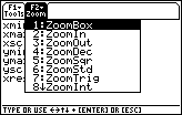
This will open a small menu box, as is shown in Figure 7. key to select the ZOOM option
shown at the top of the screen.
This will open a small menu box, as is shown in Figure 7.
|
Figure 7

| We will opt for the
ZoomStd option by pressing  .
This will set the xMin value to – 10,
xMax to 10, xScl to 1,
yMin to – 10,
yMax to 10, and yScl to 1. It also moves us back to
graph mode and a new graph, see Figure 8, will be drawn. .
This will set the xMin value to – 10,
xMax to 10, xScl to 1,
yMin to – 10,
yMax to 10, and yScl to 1. It also moves us back to
graph mode and a new graph, see Figure 8, will be drawn.
|
Figure 8

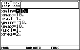
| In Figure 8 we have the new graph that uses the new WINDOW settings.
It still does not seem to correspond to the figure in the book. First, the x-axis
in Figure 8 needs to be raised. We can do this by making the yMin value more negative.
Second, the "tick" marks on the y-axis are too close together. We can alter
this by increasing the value assigned to yScl. |
Figure 9

| We move to Figure 9 by presing the 
 key to open the WINDOW
settings. A review of Figure 9 shows that we have indeed established the ZoomStd settings
described above. key to open the WINDOW
settings. A review of Figure 9 shows that we have indeed established the ZoomStd settings
described above. |
Figure 10

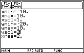
| Figure 10 shows the WINDOW settings screen after we have used the cursor keys
to move down to the yMin line, and then we entered a new value for yMin,
namely, – 20.
Then we moved to the yScl line and changed that value to be 2.
|
Figure 11

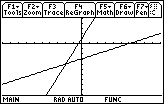
| Now, to get to Figure 11 we press the 
 key to do another graph.
This graph looks similar to the graph in the textbook. However, the graph in
the text tells us the x and y coordinate
of the point of intersection of the two lines.
We need to find the command to get the calcualtor to find that point.
A review of the menu at the top of Figure 11 does
show that we have the "Math" option available. We press the key to do another graph.
This graph looks similar to the graph in the textbook. However, the graph in
the text tells us the x and y coordinate
of the point of intersection of the two lines.
We need to find the command to get the calcualtor to find that point.
A review of the menu at the top of Figure 11 does
show that we have the "Math" option available. We press the
 key to open that option window. key to open that option window.
|
Figure 12

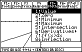
| The Math window is displayed in Figure 12.
The command that we want to use is item 5: Intersection.
We press the
 key to select that option. key to select that option. |
Figure 13

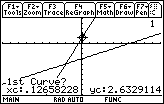
| As a result of selecting the Intersection option,
Figure 13 shows us that the
calculator is proposing that our line for y(x)=5x+2 be our first curve.
We can
examine the graph in Figure 13 and we will see that,
at the point x=.12658228, y=2.6329114, the calcualtor
has displayed a special symbol. That is how the calculator identifies the particular
line that it is proposing to use. We can press the
 key to accept that proposal.
This will move the graph to Figure 14. key to accept that proposal.
This will move the graph to Figure 14. |
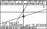
Figure 14

| Now we need to select the second curve.
The calculator is proposing the other line, y(x)=x–6,
for the second curve. The calculator is making this proposal by displaying its
flashing sign on a point, x=0.12658228, y=– 5.873418, on that line.
Again, we will accept the proposal by pressing the
 key. key. |
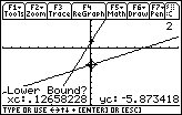
Figure 15

| In Figure 15 the calculator has been given the two curves, and now it wants a
a lower bound, the low end of the interval in which it should look for
the intersection.
The calcualtor offers the point (0.12658228,– 5.873418) as that lower bound.
We do not want to use that value. Therefore, we will continue to press the
 key to move the flashing target to the
left of the point of intersection. The result is shown in Figure 16. key to move the flashing target to the
left of the point of intersection. The result is shown in Figure 16.
|
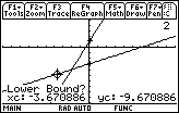
Figure 16

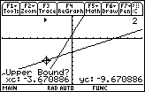
| In Figure 16 we have moved the flashing target to the left of the
point of intersection.
This new point, (-3.6708886,– 9.670886),
can be our lower bound.
Therefore, we press the
 key to accept that point. key to accept that point. |
Figure 17

| The calculator responds, as shown in Figure 17, by
asking for an Upper Bound. (In addition, the calculator has placed a
small right-pointing arrow
just below the top option line, to indicate were we have set the
lower bound.) Again the proposed point is
not acceptable. We use the
 key to move the flashing target to the
right until we have moved beyond the point of intersection. key to move the flashing target to the
right until we have moved beyond the point of intersection.
|
Figure 18

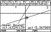
| Having moved the flashing target to the right, we are now in a position to
accept (0.63291139,– 5,367089)
as the Upper Bound. We do this
by pressing the  key. key.
|
Figure 19

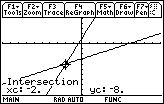
| As a result of all of our efforts, the calculator display shifts to
Figure 18. In that Figure, the calculator has identified the point of intersection
of the two lines, namely at the point
(– 2,– 8).
Even given the better resolution on the TI-89, this graph is remarkably similar to the
graph that is given in the textbook.
The major difference is that the textbook version contains the
equations of the two lines.
A closer examination of the graph in the textbook shows that these
equations were pasted into the book;
after all, the equations in the book appear in
a completely different font.
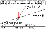
We too can doctor a picture.
We have done that in Figure 20. |
Figure 20

| You can not produce Figure 18 directly from the calculator.
The equations have been
added to this image.
In addition, we have added a red line from the point of
intersection straight up to the x-axis.
In additon, we have replaced the x-axis from directly above the point of intersection all the
way to the left by a light blue line.
This represents the
x-values where the line y(x)=5x+2 is below the line y(x)=x–6.
In effect, this is the
set of points where 5x+2 < x-6 which was the original problem. |
The material above produced a graph similar to the one given in the textbook.
The detailed TI-86 notes
for this section address the steps needed to produce a graph directly from the given
inequality, namely,
Figure 21

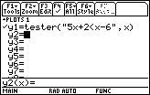
| Figure 21 returns to the y= screen via the

 keys. In this case we have cleared all of the
old functions and have added the line that you see in Figure 21, namely,
y1=tester("5x+2<x–6",x)
This is the method used to call the function
tester() and to send it the relational expression
5x+2<x–6. The additional ,x is required. keys. In this case we have cleared all of the
old functions and have added the line that you see in Figure 21, namely,
y1=tester("5x+2<x–6",x)
This is the method used to call the function
tester() and to send it the relational expression
5x+2<x–6. The additional ,x is required.
|
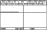
Figure 22

| In Figure 22 we graph the new function by pressing the

 keys.
We can see that the value of the function is 1
up to x having the value of negative two (– 2. At
that point the graph drops to 0, which is right on top of the x-axis.
This is a problem similar to
that seen for the TI-86. We can return to the y= screen via
the keys.
We can see that the value of the function is 1
up to x having the value of negative two (– 2. At
that point the graph drops to 0, which is right on top of the x-axis.
This is a problem similar to
that seen for the TI-86. We can return to the y= screen via
the 
 key sequence and
there we can modify the function to use
the same trick that we did for the TI-86. key sequence and
there we can modify the function to use
the same trick that we did for the TI-86.
|
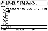
Figure 23

| Back at the y= screen, we press the
 key
to bring a copy of the y1 function into the
edit area at the bottom of the screen. Then we modify the
function so that it appears as
y1=tester("5x+2<x–6",x)*5–2
Then, we press the key
to bring a copy of the y1 function into the
edit area at the bottom of the screen. Then we modify the
function so that it appears as
y1=tester("5x+2<x–6",x)*5–2
Then, we press the
 key to accept the new definition for y1.
This leaves us with the screen appearing as in Figure 23.
Note that there is not sufficient roomn
to fully display the new function on the y1= line. key to accept the new definition for y1.
This leaves us with the screen appearing as in Figure 23.
Note that there is not sufficient roomn
to fully display the new function on the y1= line.
|
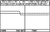
Figure 24

| In Figure 24 we graph the new function by pressing the

 keys.
Now we can see more clearly the region where the
function is true (the elevated portion of the graphed values)
and where it is false (the depressed portion of the graphed values). keys.
Now we can see more clearly the region where the
function is true (the elevated portion of the graphed values)
and where it is false (the depressed portion of the graphed values).
There does seem to be an oddity here.
The graph does not drop down from true to false immediately.
A close examination of the graph indicates that the drop happens over a few pixels.
This should not be the case.
We know that the value of the function is either 3 for TRUE or
– 2 for FALSE. What is
going on here?
|
Figure 25

| In Figure 25 we have returned to the WINDOW settings screen via the

 keys.
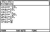
When we last saw this screen, back in Figure 10,
we did not pay any attention to the final setting, the value
assigned to xres. That values was 2.
Now, in Figure 25, we have moved down to that value and have changed it to be 1.
The xres setting determines how often the calculator will compute values from the domain of the function.
When xres was set at 2, the TI-89 would compute
function values for every second point on the graph, and the calculator would interpolate
values for the missing points.
Doing this means that the calculator only has to evaluate the
function for half of the points on the graph.
This speeds up the process of drawing the graphs. Now that we have changed the
xres setting to be 1, on any new graph
the calculator will compute the value of the function at each point on the x-axis. keys.
When we last saw this screen, back in Figure 10,
we did not pay any attention to the final setting, the value
assigned to xres. That values was 2.
Now, in Figure 25, we have moved down to that value and have changed it to be 1.
The xres setting determines how often the calculator will compute values from the domain of the function.
When xres was set at 2, the TI-89 would compute
function values for every second point on the graph, and the calculator would interpolate
values for the missing points.
Doing this means that the calculator only has to evaluate the
function for half of the points on the graph.
This speeds up the process of drawing the graphs. Now that we have changed the
xres setting to be 1, on any new graph
the calculator will compute the value of the function at each point on the x-axis.
|
Figure 26

| We return to the graph via the

 keys.
This time the drop from TRUE to FALSE is much more immediate. keys.
This time the drop from TRUE to FALSE is much more immediate. |
Figure 27

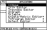
| The following 8 screens demonstrate the steps needed
to obtain a listing of the tester() function.
We start by pressing the
 keys.
This opens the window shown in Figure 27. Of these
applications, we wish to use the Program Editor. keys.
This opens the window shown in Figure 27. Of these
applications, we wish to use the Program Editor. |
Figure 28

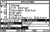
| In Figure 28 we have selected the Program Editor
by pressing the  key. This opens another window, one that asks if we want
to open the Current program, some other program, or create a new program?
We have moved the highlight to the second option, to open some other program.
Then, to perform that option we press the
 key. key.
|
Figure 29

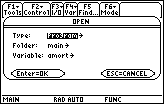
| Figure 29 shows the screen that will allow
us to choose the program that we wish to open.
In this case, we will want to open the function tester().
A function is a special
kind of program.
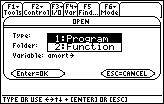
The setting for Figure 29 is to open a program. We need to change this
to open a function. Therefore, we press the
 key to open
the selection window, as shown in Figure 30. key to open
the selection window, as shown in Figure 30.
|
Figure 30

| The selection window in Figure 30 gives us the choice of
a program or a function. Naturally,
we select option 2, function, by pressing the
 key. key. |
Figure 31

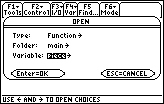
| Notice, in Figure 31, that the screen now
indicates that we are looking to open a function.
That function happens to be in the main folder,
so the next setting is correct. But the bottom setting
suggests that the name of the function that we want
to open in main is piece. We need to
change this setting. |
Figure 32

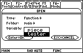
| In Figure 32, we have pressed
the  key to
look at the list of functions that we can open.
Then we have moved the highlight down to tester.
We can select that function by
pressing the key to
look at the list of functions that we can open.
Then we have moved the highlight down to tester.
We can select that function by
pressing the  key.
This will move us to Figure 33. key.
This will move us to Figure 33. |
Figure 33

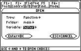
| In Figure 33 we finally have our options set appropriately. We press the
 key to
perform the task of openning the function tester in the main folder. key to
perform the task of openning the function tester in the main folder. |
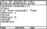
Figure 34

| Figure 34 lists the function tester. This is the text that you would have to
type into the calculator if you wanted to create your own version of
tester without downloading it from another machine or from a PC. |
