


| Note that the TI-86 and the TI-85 have slightly different keys. This page uses the keys associated with the TI-86. The differences are in the "2nd" functions on some of the keys used here. The TI-85 keys will have the same key-face symbol unless otherwise noted. |
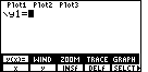
The graphical solution to Example 14 Chapter 1 Section 2 of the text is not quite as simple to construct as one might hope. That example uses the problem
|
|
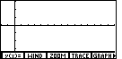
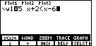
Figure 1 shows the result of pressing the |
|
| Press the |
|
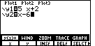
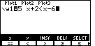
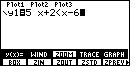
| To produce Figure 3 we have pressed the
|
|
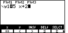
| Having entered the functions in Figure 3, we press
|
|
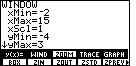
| To open the WINDOW menu we press the
|
|
| Figure 6 shows the start of the ZOOM submenu. We will opt for the
ZSTD option by pressing |
|
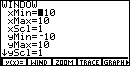
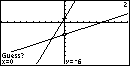
| In Figure 7 we have the new graph that uses the new WINDOW settings. It still does not seem to correspond to the figure in the book. First, the x-axis in Figure 7 needs to be raised. We can do this by making the yMin value more negative. Second, the "tick" marks on the y-axis are too close together. We can alter this by increasing the value assigned to yScl. |
|
|
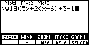
We move to Figure 8 by presing the |
|
| Figure 9 shows the WINDOW settings screen after we have used the cursor keys to move down to the yMin line, and then we entered a new value for yMin, namely, – 20. Then we moved to the yScl line and changed that value to be 2. |
|
| Now, to get to Figure 10 we press the
|
|
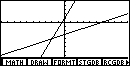
| Figure 11 shows the next five items in the menu. Now we have a interesting
choice, namely, the MATH submenu. Press
|
|
| The MATH submenu is displayed in Figure 12. Again, it does not seem to have the
command that we desire. We press the
|
|
| The middle option in the MATH submenu is ISECT, a plausible
abbreviation for INTERSECTION. We press the |
|
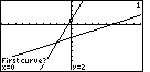
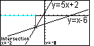
| As a result of selecting the ISECT option, Figure 14 shows us that the
calculator is proposing that our line for y(x)=5x+2 be our first curve. We can
examine the graph in Figure 14 and we will see that at the point, x=0, y=2, the calculator
has displayed a special symbol. That is how the calculator identifies the particular
line that it is proposing to use. We can press the
|
|
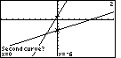
| Now we need to select the second curve. The calculator is proposing the other line, y(x)=x-6,
for the second curve. The calculator is making this proposal by displaying its
flashing sign on a point, x=0, y=-6, on that line.
Again, we will accept the proposal by pressing the
|
|
| In Figure 16 the calculator has been given the two curves, and now it wants a guess,
a starting point. In fact, the calcualtor offers the same point (0,-6) as that starting
point. We can accept that point as our guess by pressing
the |
|
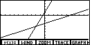
| As a result of all of our efforts, the calculator display shifts to Figure 17. In that Figure, the calculator has identified the point of intersection of the two lines, namely at the point (– 2,– 8). This graph is remarkably similar to the graph that is given in the textbook. The only difference is that the textbook version contains the equations of the two lines. A closer examination of the graph in the textbook shows that these equations were pasted into the book; after all, the equations in the book appear in a completely different font. We too can doctor a picture. We have done that in Figure 18. |
|
| You can not produce Figure 18 directly from the calculator.
The equations have been
added to this image. In addition, we have added a red line from the point of
intersection straight up to the x-axis.
In additon, we have replaced the x-axis from directly above the point of intersection all the
way to the left by a light blue line. This represents the
x-values where the line |
It might have been nice to be able to graph the original problem

|
Figure 19 returns to the "y=" screen.
The  key returned the main graph menu to Figure 18.
Then the key returned the main graph menu to Figure 18.
Then the  key will open the "y=" screen.
For this example we have
deleted any existing function definitions in that screen, using the key will open the "y=" screen.
For this example we have
deleted any existing function definitions in that screen, using the
 
  . That leaves us with the challenge
of producing the "less than" sign, which does not appear on the keyboard. . That leaves us with the challenge
of producing the "less than" sign, which does not appear on the keyboard.
|
|
To produce the "less than" sign we press the  keys to open the TEST menu shown in
Figure 20. This menu gives us the option of choosing the "less than" character.
keys to open the TEST menu shown in
Figure 20. This menu gives us the option of choosing the "less than" character.
|
|
Figure 21 completes the function by pressing  to select the "less than" character from the menu, and then

 to finish the line. to finish the line.
At this point we note that the option to GRAPH has been lost from the menu scheme. |
|
We press to close the bottom menu of Figure 21 and
therefore to produce Figure 22.
|
|
Rather than just make the graph of our function, we will use the
ZOOM menu options to change the WINDOW settings. Therefore,
we use the  keys
to change the menu structure to that shown in Figure 23. Then,
we press keys
to change the menu structure to that shown in Figure 23. Then,
we press  to select the
STANDARD settings and move immediately to Figure 24. to select the
STANDARD settings and move immediately to Figure 24.
|
|
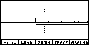
Figure 24 shows the graph of the the inequality, where every x-value that
makes the inequality true is associated with the y-value 1, and every
x-value that makes the inequlity false is associated with the y-value 0.
Unfortunately, graphing the y-value 0 merely puts the graph on top
of the x-axis. This makes it hard to see. We can modify the orginal function to improve the visibility of the function. |
|
We return to the y= screen via the key.
We know that the expression  will shift the calculator into insert mode. Then, press the
  to generate the initial left parenthesis.
Then move to the right end of the expression by pressing the
|
|
Pressing  moves the
calculator from Figure 25 to Figure 26. Here we can see just where the expression is true, i.e.,
where it has the value 2, and where the expression is false, i.e., has the value – 1. moves the
calculator from Figure 25 to Figure 26. Here we can see just where the expression is true, i.e.,
where it has the value 2, and where the expression is false, i.e., has the value – 1.
|

|
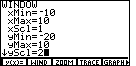
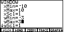
Knowing that the graph ranges from 2 to – 1, we can return to the WINDOW
screen, via the key, where we can change the
values for yMin and yMax. Figure 27 shows the screen with the settings
generated by our ZOOM Standard, back in Figure 23.
|
|
In Figure 28 we have changed the settings. After making the appropriate changes, we can press
to move back to the graph, as shown in Figure 29.
|
|
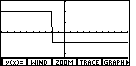
The graph has changed as a result of our changes in the yMin and yMax values.
It is now even easier to see the change from true (the value 2) to false (the value – 1).
At the same time the almost vertical line connecting the true values to the falsw values has become even more
prominent. That nearly vertical line is not part of the graph. At no time does
|
|
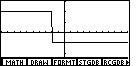
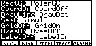
To turn off the setting we need to move to the FORMT command in the menu.
FORMT is not shown in the menu of Figure 29. However,
if we press the  key, the menu changes to that shown in
Figure 30. Now we can use the FORMT command by pressing
the key. key, the menu changes to that shown in
Figure 30. Now we can use the FORMT command by pressing
the key.
|
|
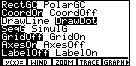
The FORMT command opens the window shown in Figure 31. We are interested in the third
line where we have two settings,
DrawLine and DrawDot. The setting shown in Figure 31 indicates that the
calculator is in the DrawLine mode, since that is the option that is highlighted.
We use the cursor keys to move down to the third line and then over to the DrawDot
option.
Once there, we press the  key to select that option. The result is
shown in Figure 32. key to select that option. The result is
shown in Figure 32.
|
|
Now that we have changed the option to DrawDot, we
can press to graph the function again, but this time with the new option set.
|
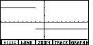
| Figure 33 shows the new version of the graph. Note that there is no longer a connecting line between the true values and the false values. |
PRECALCULUS: College Algebra and Trigonometry
© 2000 Dennis Bila, James Egan, Roger Palay
 key, and finish the expression
with
key, and finish the expression
with 


 .
.