Simplex Method Using the TI-85/86 SM2 Program

This page demonstrates the use of the TI-85/86 program SM2 to perform the Simplex Method. The page steps through the keystrokes and resulting screens for solving two linear programming problems. These problems are taken directly from the textbook.

Before using the SM2 program, it must be loaded onto your calculator. This can be done in class by linking calculators and downloading from one to another.

Note that the first 10 screens (Figures) below are directly related to the TI-85 only. These screens are included here because the TI-85 has a much smaller memory space than does the TI-86. It is likely that memory size may become a problem with the TI-85. Therefore, Figures 1 through 10 demonstrate examining the available memory space on the TI-85. There are similar features on the TI-86, but it uses slightly different keys.

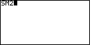
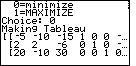
Figure 1 (TI-85 Memory Check)	Before we even begin to use the SM2 program on the TI-85, and perhaps even before we load the SM2 program onto the TI-85, we need to make sure that there is sufficient space for the program and the storage it requires. To do this we look at the memory status of the TI-85. The keystrokes Open the window shown in Figure 1.
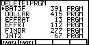
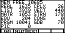
Figure 2 (TI-85 Memory Check)	The first thing that we need to do is to see the current Random Access Memory (RAM) allocations. To do this, from Figure 1, press the key. This will display a version of Figure 2. Note that the values in Figure 2 are from a particular calculator at a particular time; they will be different from the values on your calculator screen. In Figure 2 we see, for example, that we have 10,685 free cells, that we have used 3939 cells to store LISTs, and that we have used 10,041 cells to store programs. The 10,685 free cells are quite enough for us. However, let us take this opportunity to examine and possibly remove an old program to create more open space.
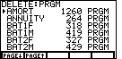
Figure 3 (TI-85 Memory Check)	We leave Figure 2 by pressing the key to select the DELET option from the menu. The result is shown in Figure 3. Now we need to decide what kinds of things we want to delete. We want to examine, and possibly delete, a program, but programs are not listed in the menu shown in Figure 3.
Figure 4 (TI-85 Memory Check)	We press the key to show additional commands in the menu option line. This results in Figure 4. Now the fifth option is PRGM. This is the option we want, so we press the key to move to Figure 5.
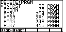
Figure 5 (TI-85 Memory Check)	Figure 5 displays the start of the list of programs that are installed on this calculator. each program is listed along with the size of the program. A small arrow, at the left of the screen, points to one program. In Figure 5, that arrow is pointing to the AMORT program. Extreme care should be taken here. The selected program will be deleted if the ENTER key is pressed. The cursor keys can be used to move the selection arrow tro another program. And the first two function keys, F1 and F2, can be used to move the display a page at a time. We will press the key to move down to the next page of the display, shown in Figure 6.
Figure 6 (TI-85 Memory Check)	Figure 6 shows more of the programs currently installed on this calculator. Note the size of the programs. The smallest program, EFFRAT, takes all of 13 locations. The largest one on Figure 6 is DOLLAR, taking 415 locations. A review of these programs does not indicated any particular one that we would want to eliminate. Therefore, we press to move to yet another page of the display, in Figure 7.
Figure 7 (TI-85 Memory Check)	Here we have more programs, but none that we want to eliminate. Press to move to the last programs, shown in Figure 8.
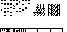
Figure 8 (TI-85 Memory Check)	The final programs on this calculator appear in Figure 8. The selection arrow, at the extreme left of the screen, was pointing to the PRSNTVAL program, which we want to keep. The next program, SIMPLEXA, taking up 803 locations, is not needed. We will pressed the key to moved the selection arrow to point to the SIMPLEXA program. This is the condition shown in Figure 8. Our next step will be to press the key to DELETE the selected program, in this case, SIMPLEXA. This will move us to Figure 9.
Figure 9 (TI-85 Memory Check)	Figure 9 shows the result of DELETING the SIMPLEXA program. It has disappeared from the list and from the calculator. It can not be retrieved.
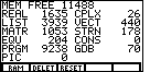
Figure 10 (TI-85 Memory Check)	We leave Figure 9 via the key. This will return us to the normal calculator screen. However, we will press the keys to re-examine the memory status, and then press to display the RAM allocations. The Figure 10 display can be compared to the Figure 2 display. PRGM memory has decreased from 10,041 to 9,238 and the FREE memory has increased from 10,685 to 11,488. We conclude our memory inspection by pressing the key to return to the normal calculator screen.

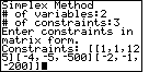
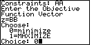
The problem that we will solve on the calculator is taken from page 233 of the text.

Figure 11	We request the SM2 program by pressing the keys to generate Figure 11. Now press the key to actually start the program.
Figure 12	The program begins by clearing the screen and then asking for the number of variables. We respond with . Then the program asks for the number of constraints. Our problem has 3 constraints. Therefore, press . And finally, in Figure 12, the program asks for the constraints in matrix form.

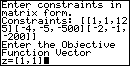
We need to give the program the constraints in matrix form. We can do this in two different ways. First, we can merely type the matrix using the "[" and "]" characters. This is the method that we will use immediately below. Second, if we had stored the matrix earlier under a name, then we could just enter the name. We will use that method for the second problem, starting in Figure 30.

Right now, we need to remember how to create the augmented matrix for the constraints. To do this we will re-write the constraints with each variable represented in the inequality. (Note: we are not adding the "slack variables" here; the program will do that for us. We are just making sure that each variable appears in each inequaltiy.]

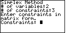
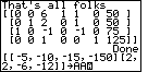
Figure 13	For Figure 13, we enter the constraints as a matrix via the keys
Figure 14	We complete Figure 13 by pressing the key. The program now asks for the "Objective Function Vector". A vector is somewhat like a list, but it has different operations and properties from a list. On the calculator, a vector is created using the square braces. For our problem, that objective function vector is made up of the objective function coefficients. Since our objective function is z = 1x1 + 1x2 the vector would be [1,1]. We enter this via the keys . This produces the text seen in Figure 14.
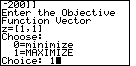
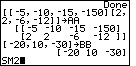
Figure 15	Pressing to accept the objective function vector of Figure 14 produces the minimize vs. MAXIMIZE choice. We select the MAXIMIZE option by pressing the key to complete Figure 15.
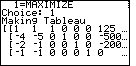
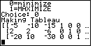
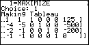
Figure 16	After Figure 15 we have given the program all of the data that it needs to do the problem. We press the key to start the process. Along the way the calculator will display intermediate results. At times it will pause to let us read those results. The first pause is shown in Figure 16. Here, the calculator has created the TABLEAU and is displaying it for us. Note that the entire matrix does not fit on the page. The three dots (...) at the right side of lines indicates that there is more to be displayed.
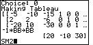
Figure 17	We have moved from Figure 16 to Figure 17 by pressing the right cursor key, , to move over on the display. The resulting TABLEAU should be compared to the one in the text at the top of page 234.
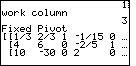
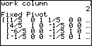
Figure 18	The calculator was paused at Figure 17 to allow us to examine the TABLEAU. We did so, and then we press the key to continue the program. The calculator entered the "Preprocessing" phase of the algorithm. In that phase, the calcualtor identified the second row as the work row (not shown), and within that second row, it identified the second column as the work column. That means that the value that was in row 2 column 2, namely -5, becomes a pivot point. Therefore, we use the second elementary row operation to change it to a 1, and the third elementary row operation to convert all remaining elements in the second column to be 0. The calculator has done exactly that, and it has paused at that point to display the resulting matrix, shown in Figure 18. This matrix corresponds to the one in the middle of page 234 in the text.
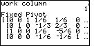
Figure 19	We leave Figure 18 by pressing the key to continue the program. The calculator continues the preprocessing phase, identifying the third row and first column as the work row and column. It then changes the pivot point to a 1, and converts the remaining work column values to 0. Again, we pause to examine the matrix, shown in Figure 19. This matrix corresponds to the bottom matrix on page 234.
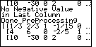
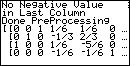
Figure 20	The key continues the process. The program looks at the matrix and determines that we are done with the preprocessing phase. It indicates that fact in the message on Figure 20, and it displays the same matrix again.
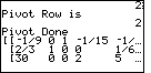
Figure 21	The key leaves Figure 20 and moves the calculator into the basic algorithm. Here the calculator determines that the fourth column is the work column, and that the first row is the work row. The calculator makes the element in row 1 column 4 become 1 and the calculator uses that 1 to change the other elements in that column to be 0. Once this is done, the calculator displays the resulting matrix and pauses to allow us to examine it, as shown in Figure 21.
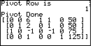
Figure 22	Pressing the key continues the algorithm. The calculator determines that we are done. It gives the message that the final matrix is being displayed and it pauses as in Figure 22.
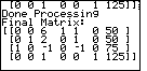
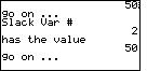
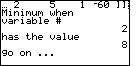
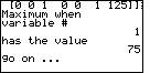
Figure 23	Now we can get the calculator's best guess at the results by pressing the key. The program responds by indicating that the maximum value for the objective function can be found when x1 has the value 75. This is exactly the value presented in the second sentence of the paragraph at the bottom of page 234. The other values follow in Figures 24 and 25, with the value of the objective function being given in Figure 26.
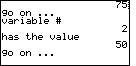
Figure 24	We continue by pressing the key, to find, in Figure 24, that the value of x2 needs to be 50.
Figure 25	Another key shows us Figure 25, whcih gives us s2, the second slack variable, having the value 50.
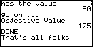
Figure 26	Yet another key moves us to Figure 26, which repeats that the objective function value will be 125.
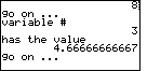
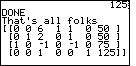
Figure 27	For a convenience, the program continues, after a press of the key, to redisplay the matrix, as shown in Figure 27. The program is paused at that point so that we can scroll over on the matirx if need be. In this case the entire matrix is displayed on screen so we do not need to scroll at all.
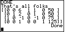
Figure 28	And, finally, another key sends the program to its end. This leaves the screen as in Figure 28.

One of the problems with the approach shown above is that there is no asy recovery if you have made an error in the original matrix, or in the objective function vector. The program merely continues, and probably produces the wrong answers. It is much safer for us to store the constraint matrix and the objective vector on the calculator before we use SM2. That way, if an error is found, we can correct it and rerun the program without having to re-enter all of the coefficients and constants. We will demonstrate this in the remaining Figures.

The next example is taken from page 238 of the text. In this case there are three variables and two constraints. The problem is stated as:

Figure 29	The first step is to create the constraint matrix. The key strokes enters the matrix. To save it under a name we use the key followed by the desired name. In the example shown in Figure 29, that name is AA and was created via the key sequence.
Figure 30	Press the key to accept the matrix of Figure 29. In Figure 30 we will enter the objective vector and save it under the name BB. A small warning: this is not the right set of values, but we will enter them here, use them, discover our error, correct them, and rerun the program with the correct values. The keys produce the vector. Note the single left and right square bracket. Then we store the vector in BB via the keys and . We finish Figure 30 by typing the name of the program, using the key sequence: .
Figure 31	The program starts as before, asking for the number of variables, , the number of constraints, , and then the matrix of constraint coefficients and constants. In this case, we have already entered that matrix and we have saved it under the name AA. Therefore, we type the name of the matrix via the keys. After that we should have a display identical to Figure 31.
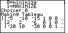
Figure 32	We leave Figure 31 by pressing . The program asks for the Objective Function Vector. Again, we have entered this and saved it under the name BB. Therefore, press and . The program moves on to ask if we want to minimize or maximize? We respond with for minimize. All of this should produce Figure 32.
Figure 33	We press to start the process. The program creates the TABLEAU and displays it, as in Figure 33. We can compare this to the matrix on page 239. It is almost the same. However, we note that the signs on the values in the bottom row are reversed. What happened? If we go back we will find that we created the objective function vector using the equation Z = -20x1 + 10x2 - 30x3 We created Z = -z as was done in the book. However, the program, SM2, does this for us when we select the "minimize" option. Therefore, SM2 has undone our conversion, and the values in the final row of the TABLEAU have the wrong sign. We need to stop the program, change the vector and then run the program again with the new vector.
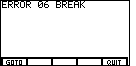
Figure 34	We stop the program by pressing the key. The calculator responds with Figure 34. We know what we need to do, and that does not involve changing the program. Therefore, we want to select the QUIT menu item. To do this we press the key.
Figure 35	Figure 35 demonstrates that we are out of the program and back to the normal calculator screen.
Figure 36	In the middle of Figure 36 you can see the steps taken to reverse the signs on the values stored in BB. Namely, we multiply -1 times BB and store the result in BB. The keys needed to do this are . The calculator multiplies each element of the vector by -1 and stores the resulting vector in BB, and displays the new BB. Now all we need to do is to start the program again. We use the keys to generate SM2 to complete Figure 36.
Figure 37	The program restarts. We answer the questions again.
Figure 38	Figure 38 shows more answers.
Figure 39	With Figure 39 we have returned to the spot where we found our original error. Now we look at the initial TABLEAU and verify that it has exactly the values that we expect.
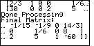
Figure 40	The key moves us to Figure 40, which shows the matrix after having made row 1 column 3 the pivot element. The matrix now checks with the one in the middle of page 239.
Figure 41	In Figure 41 we find that the program has determined that we are done with the preprocessing.
Figure 42	Figure 42 shows the matrix after the next step. It now corresponds to the matrix at the bottom of page 239.
Figure 43	The program announces, in Figure 43, that we are done, and it redisplays the matrix.
Figure 44	Figure 44 continues the display from Figure 44, except that we use the key a number of times so that we can see the right side of the matrix.
Figure 45	The program now steps through what it believes to be the solution. In Figure 45 we have the statement that x2 is 8.
Figure 46	Figure 46 has x3 being 4  2/3, or 14/3.
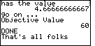
Figure 47	And, Figure 47 shows the objective value to be 60.
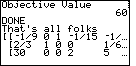
Figure 48	A final display of the matrix shows up in Figure 48. The program is still running. It is just PAUSED. Therefore we can use the cursor key to move around in the matrix.
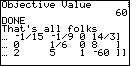
Figure 49	Here, in Figure 49, we have moved again to the right side of the matrix.
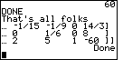
Figure 50	One last key finishes off the program and returns us to the normal calculator mode.