Matrix Operations for the TI-89: Examples from text, page 135

MATRIX OPERATIONS

Matrix Operations for the TI-89: Examples from text, page 135

This page is devoted to presenting, in a step by step fashion, the keystrokes and the screen images for entering and manipulating matrices on a TI-89, at least up to the point of doing all of the problems from 7 through the first few parts of problem 58 on page 135 of the textbook. These problems are based on the matrices that appear in the text:

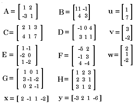
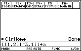
Figure 1	Although we could use the Data/Matrix Editor to enter these matrices, we will use the simple data entry technique here. To do this we need to enter each matrix using the [ and ] characters to represent the start and end of the matrix, as well as represent the start and end of each row of values. We use a comma to separate values. Thus, to enter the matrix A in the book we enter the line [[1,2][-3,1]] and then we want to STOre the result in the variable a. Figure 1 shows the line as we have entered it. Note that the TI-89 is not case-sensitive. That is, the variable A and the variable a are identical. In fact, the TI-89 will change the variable A into a. Therefore, in choosing the names for the matrices, this example merely uses the lowercase version of each letter name.
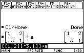
Figure 2	In Figure 2 we have pressed the key. The calculator responds by placing our command on the left of the HOME screen, and the result on the right, both above the command line. We immediately note that the calculator has employed its "prettyprint" routines to "clean up" our entry. The matrix actually looks like a matrix, without the left and right square brackets that we used for data input.
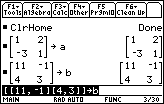
Figure 3	Figure 3 shows the HOME screen after we have entered the second matrix and assigned it to b and pressed the key.
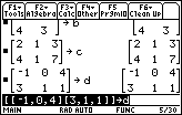
Figure 4	Most of the remaining matrices are entered the same way. As new matrices are entered, the display scrolls off the top of the screen. Thus, Figure 4 shows the subsequent entry of both c and d, but the [4, 3 ] at the top is left over from the end of the display of the b matrix. Note that for these matrices, c and d, there are three numbers in each row.
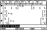
Figure 5	Although the calculator may allow some less formal way of entering u and v, Figure 5 follows the strict pattern established above for a, b, c, and d. That is, we start each matrix with [, we enter each row as [ followed by a set of numbers separated by commas and ending with ], and we end the matrix with ]. For matrix u there is only one number per row. The same is true for matrix v.
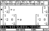
Figure 6	Figure 6 shows the entry for matrix e, which has three rows, but only two elements (numbers) in each row.
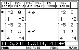
Figure 7	Figure 7 shows the entry for matrix f, which also has three rows, but only two elements in each row.
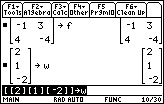
Figure 8	Figure 8 displays the entry of matrix w. This follows the pattern for both matrix u and matrix v in that there is only one element per row. However, for matrix w there are three rows.
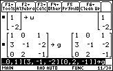
Figure 9	Figure 9 displays the entry of matrix g, the largest matrix so far with three rows and three columns. Matrix g is so large that the input (coomand) line scrolls off on the left side as we enter the last few characters of the matrix. The three dots at the left indicate that part of the command is no longer visible.
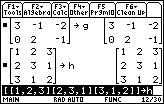
Figure 10	Figure 10 shows the results of entering matrix h.
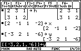
Figure 11	Both matrix x and matrix y have been entered in Figure 11. As you can see, the formal way of entering each of these matrices is to mark the start and end of the matrix, as before, with the [ and ] characters. We also enclose the one and only row in each matrix with another set of [ and ] symbols. THe command line for matrix y is still visible in Figure 11.
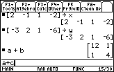
Figure 12	Now we are ready to do the problems that are in the book. To do problem 7 press and to generate a+b. Then press to perform the addition. The sum of the two matrices is displayed. This is shown in the middle of Figure 12, at the right side of the screen. Going back to the original values of a and b it is easy to see how a+b is formed. *The new matrix looks like the original ones, but each element of the answer is the sum of the corresponding elements of the original matrices.* We finish Figure 12 by stating the addition of problem 8. 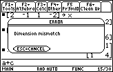We do this by pressing and to generate A+C. When we press to submit a+c and the result is Figure 13.
Figure 13	Figure 13 displays an error message box. The error is the result of our command a+c. We can not add matrices unless they have the same number of rows and columns. Matrix a is a 2x2 matrix (2 rows and 2 columns), but matrix c is a 2x3 matrix [2 rows and 3 columns]. Therefore, addition of a and c is not defined, and our attempt to add the two matrices causes the error. We can press to select the CANCEL option.
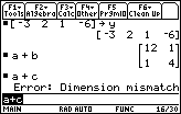
Figure 14	Once we have canceled the action we ware returned to the HOME screen, shown in Figure 14. Note that the calculator has made note of the fact that we had an error. We are now free to edit the offending command, or to replace it with a new command. We have our answer for problem 8, namely, "it is not legal to add a and c.
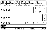
Figure 15	In Figure 15 we have gone on to add matrx c and matrix d, both have two rows and three columns. We say that each is of "order 2x3". Thus we should be able to add them, as required in problem 9. And, we have added matrix u to matrix v, each of which have two rows and one column. And we finished with x+y, where the two matrices each have one row and four columns.
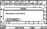
Figure 16	Figure 16 represents an attempt at doing problem 12, u+y. Unfortunately, u is of order 2x1 whereas y is of order 1x4. Therefore, we can not add them, and the calculator refuses to do our command.
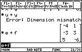
Figure 17	Figure 17 shows the remains of the error in Figure 16 and problem 13 (e+f), which works.
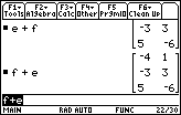
Figure 18	Figure 18 shows the result of problem 14 (f+e). It It is important to note that problems 13 and 14 demonstrate the fact that matrix addition is COMMUTATIVE. That is, there is no difference between e+f and f+e. The last portion of the answer to problem 13 is seen at the top of the screen, while the answer to problem 14 is seen at the bottom. The answers are identical.
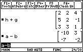
Figure 19	Figure 39 shows the result of doing h+g and the result of problem 16, a-b. We can verify that subtraction of matrices is similar to addition of matrices. The answer is the same "order" as the original matrices, and each element of the answer is the difference of corresponding elements of the original matrices.
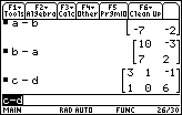
Figure 20	Since subtraction of numbers is NOT commutative, we would not expect the subtraction of matrices to be any different. Figure 20 verifies this. It shows the results of both a-b and b-a. The two answers are opposites of each other, just as 7-4 and 4-7 generate opposite answers. In addition, Figure 20 contains the result for Problem 18, c-d.
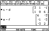
Figure 21	We want to compare Figure 21 with Figure 22. Again, we have a demonstration showing that subraction is not commutative. In Figure 21 we have e-f.
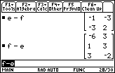
Figure 22	Figure 22 demonstrates that we get different answer for f-e.
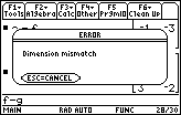
Figure 23	Again, both addition and subtraction require the matrices to be of the same order. In Figure 23 we try to perform f-g, but f is of order 3x2 and g is of order 3x3. As a result, the calcuator reports that it can not perform the operation.
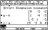
Figure 24	We can, however, perform g-h and x-y.
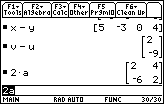
Figure 25	Figure 25 completes the subtraction examples with v-u. It then demonstrates the multiplication of a matrix by a numeric constant. This is called scalar multiplication. In this case, we multiply matrix a by the constant 2. Comparing the result with the matrix stored in a shows that multiplying a matrix by a constant produces a new matrix, of the same order, with each element of the matrix multiplied by the constant. Note that the calculator recognizes implied multiplication here. The key strokes were . We did not need to use the multiplication key.
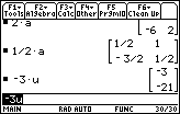
Figure 26	Two more scalar multiplication problems are demonstrated in Figure 26. Note should be made about the danger of writing 1/2a. The calculator has performed the operation properly. However, it would have been safer to have entered the problem as (1/2)a, making sure that we produce the value of 1/2 and then multiply that times the matrix a.
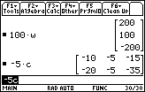
Figure 27	Here we continue with examples of scalar multiplication.
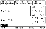
Figure 28	Problem 31, shown in Figure 28, introduces a more complex expression involving both subtraction and scalar multiplication. As we might expect, for the problem a-2b, the scalar multiplication is done first and the result is subtracted from matrix a to produce the final result.
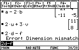
Figure 29	Figure 29 illustrates a successful evaluation of 2u+3v and an error in the attempt to perform 2d-f. That error is caused by the fact that 2d is of order 2x3 whereas f is of order 3x2. Figure 29 represents the calculator screen after we have left the pop-up error message.
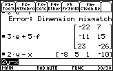
Figure 30	Problems 34 and 35 produce successful results in Figure 30.
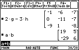
Figure 31	Figure 31 starts with another example of combining scalar multiplication with subtraction in problem 36, 2g-3h. Figure 31 then demonstrates problem 37 which calls for the multiplication of two matrices. In the book the problem is written as AB, where we understand the implied multiplication. The calculator recognizes names such as AB as two character variables. Therefore, unlike scalar multiplication, we need to use the multiplication symbol to indicate the operation. We press and the calculator displays *ab**. Then, we conclude the command with the key. The calculator performs the operation and displays the result as shown in Figure 31.

We need to stop here and examine the result of the multiplication of two matrices. The resulting answer is not as clear as it was for matrix addition, subtraction, scalar multiplication, or a combination of these. To perform a matrix multiplication each element of the answer is formed by obtaining the sum of the products of the elements of the corresponding row of the first matrix with the elements of the corresponding column of the second matrix. In Figure 31, the 5 in the answer is in row 1 column 2. Therefore, the 5 came from adding up the products of multiplying each element of row 1 of the first matrix, a, with each element of column 2 of the second matrix, b. The first row of a was 1 2. The second column of b was -1 3. We multiply 1*(-1) and 2*3, to get -1 and 6, which we add to get 5, the element in row 1 column 2 of the answer. This process is pictured in the next 4 figures.

Figure 31a	Multiply row 1 of a times column 1 of b to get row 1 column 1 of the answer.
Figure 31b	Multiply row 1 of a times column 2 of b to get row 1 column 2 of the answer.
Figure 31c	Multiply row 2 of a times column 1 of b to get row 2 column 1 of the answer.
Figure 31d	Multiply row 2 of a times column 2 of b to get row 2 column 2 of the answer.

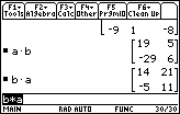
The discussion above about multiplying two matrices is clouded by the fact that the two we are using, a and B, are square, that is, they each have the 2 rows and 2 columns. As we will see later, matrix multiplication has some curious restrictions and consequences.

Figure 32	In Figure 32 we can see one immediate consequence of our definition of matrix multiplication. In particular, Figure 32 shows both *ab** and ba. We can see that these two do not produce the same results. Whereas multiplication of numbers is commutative, in general, the multiplication of matrices is not commutative*.
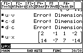
Figure 33	Figure 33 shows the result of four problems, 39-42. The first three are unsuccessful. In particular, we can not multiply u and v, nor can we multiply c and d. We have seen that we could have added u and v, or c and d, because each pair has the same order. Why can't we multiply them? When we multiply matrices the number of columns of the left matrix must match the number of rows of the right matrix. In Figure 32, for *ab and ba* this was not a problem since these are square matrices and both have 2 rows and 2 columns. But u is a 2x1 matrix and so is v. Thus, u has 1 column, but v has 2 rows. Matrix multiplication is not defined in such a case. Problem 40, CD, does not work because the 3 columns of c do not match the 2 rows of d. Problem 41, DC, does not work because the 3 columns of d do not match the 2 rows of c. Problem 42, UX, works since the 1 column of u matches the 1 row of x. It is worth your time to verify this multiplication by hand.
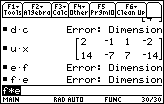
Figure 34	Problem 43, EF, does not work because the 2 columns of e do not match the 3 rows of f. Problem 44, FE, does not work because the 3 columns of f do not match the 2 rows of e.
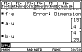
Figure 35	Figure 35 shows the successful matrix multiplication of *au and bu*. In both cases, the left matrix has 2 columns and the right matrix has 2 rows.
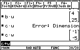
Figure 36	Problem 47, Cu, does not work: C has 3 columns and u only has 2 rows. However, Problem 48, Cw, does work: C has 3 columns and w has 3 rows. We should note here, that the answer has the same number of rows as did the left matrix and the same number of columns as did the right matrix. In this case, C has 2 rows and w has 1 column, so the answer is of order 2x1.
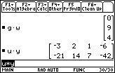
Figure 37	We can multiply a 3x3 matrix times a 3x1 matrix. This produces a 3x1 matrix. And, in Figure 37, we see that a 2x1 matrix multiplied times a 1x4 matrix produces a 2x4 matrix.
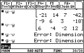
Figure 38	In Figure 38, after successfully multiplying *vy**, we find the expected errors in problems 52 and 53.
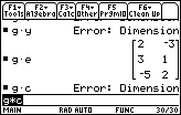
Figure 39	*ge works, but gc* does not.
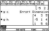
Figure 40	And, of course, since g and h are both 3x3, we can multiply *gh**.
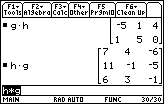
Figure 41	And we can multiply *hg, but we get a different result than we had in Figure 40 for gh*.
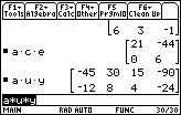
Figure 42	Figure 42 shows the beginning of some work on problem 58. That problem did not ask us to actually multiply the matrices, but it is nice to see that the calculator has no problem doing just that. It is clear that the order of *ace* is 2x2, and that the order of *auy* is 2x4.
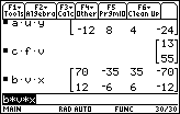
Figure 43	Figure 43 continues the work on portions of problem 58. Knowing that the multiplications work, it is worth the time to go through these and make sure that you could predict the size of the answer from the sizes and order of the original matrices.