| Table of Figures and Explanations | |||||||||||||||||||||||||||||||

|
We will start solving the problems posed above using the FINANCL program.
To do this we need to start the program. We use the
 key to open
the list of programs. The calculator used to generate these particular screens
had numerous programs on it. We use the key to open
the list of programs. The calculator used to generate these particular screens
had numerous programs on it. We use the  key
to move the highlight down to point to the FINANCL program.
Once highlighted, we select that program by pressing
the key
to move the highlight down to point to the FINANCL program.
Once highlighted, we select that program by pressing
the  key, moving to Figure 2. [Note that since this program has been
enumerated by this calcualtor as the 9th
program we could have selected it via one keystroke by pressing the key, moving to Figure 2. [Note that since this program has been
enumerated by this calcualtor as the 9th
program we could have selected it via one keystroke by pressing the
 key.] key.]
| ||||||||||||||||||||||||||||||
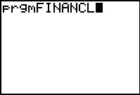 |
Selecting the program, as we did in Figure 1, does not run the program. Rather,
it pasts the name of the program following the special code "prgm" onto the screen,
as shown in Figure 2.
Now. to run the program we press .
Return to description table. | ||||||||||||||||||||||||||||||
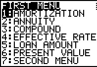 |
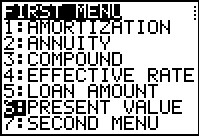
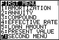
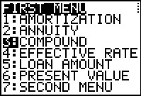
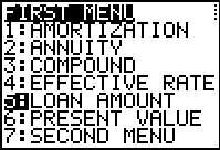
This particular program is menu driven. That is, the program displays a menu and the user
needs to choose one of the options available on that menu. Note that the entire menu must
fit on the screen. Therefore, there is a limit of 7 choices. If we want more than 7 choices,
which we do in this case, we need to create multiple menus. As we will see later,
item 7 of this menu takes us to a second menu for more choices.
The FUTURE VALUE problem is handled as a simple COMPOUND interest problem. Thus, the choice we want it item number 3. | ||||||||||||||||||||||||||||||
 |
We use the key to move thee highlight to item 3 and
then press the key to actually request that item.
| ||||||||||||||||||||||||||||||
 |
To solve the typical COMPOUND interest problem, the program asks for the PRESENT VALUE. | ||||||||||||||||||||||||||||||
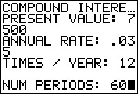 |
In Figure 6 we have given the program the value 7500
and then we press the key.
The program responds by asking for the ANNUAL RATE, to which we enter .035 (for 3.5%).
Then the progarm asks for the number of compounding periods in a year (TIMES / YEAR),
and we specify 12 for monthly. Finally the program asks for the NUMber of PERIODS
to which we respond 60 (that being 5*12). At this point we have given the program all
the information it needs. Once we press the key
the program will do the required computations and then display the answer.
| ||||||||||||||||||||||||||||||
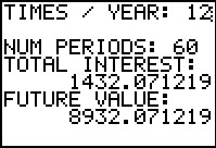 |
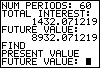
The program was nice enough to not only compute the final answer (8932.071219, which we round to 8932.17)
but also to compute the amount of interest earned, 1432.071219. The program then
waits on this screen so that we can read the answer.
[Jump to Figure 45 to see the same answer from the TVM Solver.]
In order to continue the program we need to
oress the key.
Return to description table. | ||||||||||||||||||||||||||||||
 |
Having finished the previous problem, the program returns to our menu. The next
problem is a PRESENT VALUE problem, and we have moved the highlight down to the PRESENT VALUE
option. Then we press the key to perform that option.
| ||||||||||||||||||||||||||||||
 |
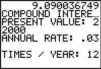
Screen 9 shows, in its last two lines, the begining of the information exchange related to the PRESENT VALUE problem. In particular, the top 6 lines are left over from our previous calculations. In the last two lines the prograqm has printed the problem type (PRESENT VALUE), and then it has asked us for the FUTURE VALUE. | ||||||||||||||||||||||||||||||
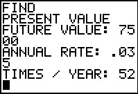 |
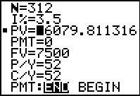
In Figure 10 we have not only given the FUTURE VALUE as 7500, we have also responded to the prompts for the ANNUAL RATE and the TIMES / YEAR with .035 and 52 (for weekly). | ||||||||||||||||||||||||||||||
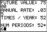 |
Figure 11 demonstrates that we can supply values as calculations, not just as numbers. Thus, in Figure 11, we have indicated that the number of periods is 52*6 rather than 312, letting the calculator do the computation. | ||||||||||||||||||||||||||||||
 |
Once we press the key to leave Figure 11 the
program computes and displays the result, namely that the PRESENT VALUE
is 6079.811316, which we can round to 6079.81.
[Jump to Figure 47a to see the same answer from the TVM Solver.]
As usual, once we have read the result we press the key
to have the program move ahead. In this case that means returning to the menu
as shown in Figure13.
This is a good place to point out that it would be a simple change to have the program round the answer for us. If we were using this program for an accounting class, that would make perfect sense. Since this is a math class I have left the values showing the full precision of the calculator computations. | ||||||||||||||||||||||||||||||
 |
The next problem, Find the Rate, does not correspond to any of the choices in the first menu.
Thus, we have highlighted the command to jumpt to the second menu.
Press the key to perform that option.
| ||||||||||||||||||||||||||||||
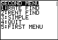 |
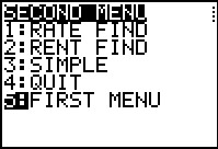
We now see the second menu. In this menu we have the RATE FIND option and we select that to move to Figure 15. | ||||||||||||||||||||||||||||||
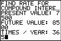 |
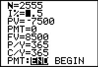
Figure 15 has the start of the data input for this problem. We have entered the values of 7500 for Present Value, 8500 for Future Value, and 365 for daily compunding. | ||||||||||||||||||||||||||||||
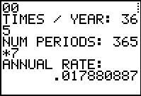 |
Here we finished the data input with 365*7 for the number of days in 7 years.
The program responded with the result .017880887 or, approximately, 1.8%.
[Jump to Figure 49 to see the same answer from the TVM Solver.]
Return to description table. | ||||||||||||||||||||||||||||||
 |
Having finished in Figure 16, the program returns to the second menu. Our next problem
is to find the Effective Rate, but that was on the first menu. We highlight option 5
and press the key to return to the first menu.
| ||||||||||||||||||||||||||||||
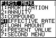 |
Back on the first menu, we have selected the EFFECTIVE RATE option. | ||||||||||||||||||||||||||||||
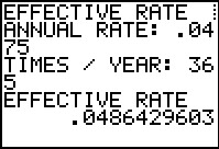 |
For EFFECTIVE RATE we only need two values, the
annual rate for the compound interest and the frequency of compounding. Both
are supplied in Figure 19 and the program responds with
the answer .0486429603 or about 4.86%.
[Jump to Figure 50 to see the same answer from the TVM Solver.]
Return to description table. | ||||||||||||||||||||||||||||||
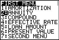 |
For Figure 20 we have returned to the main menu where we are prepared to select item 2: ANNUITY. | ||||||||||||||||||||||||||||||
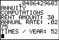 |
Figure 21 shows that we have entered the first three values, the rent amount, the annual rate, and the frequency of payments (and compounding) in a year. | ||||||||||||||||||||||||||||||
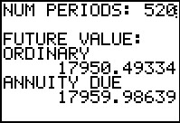 |
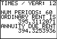
Here we have supplied the final information, the number of periods.
The program then computes and displays the two answers, one for an ORDINARY annuity
where payments are made at the end of each period
(17950.49334) and the other for an ANNUITY DUE (17959.98639) where payments are made
at the start of each period.
[Jump to Figure 52 to see the same
ORDINARY annuity answer from the TVM Solver.]
[Jump to Figure 54 to see the same
Annuity DUE answer from the TVM Solver.]
Return to description table. | ||||||||||||||||||||||||||||||
 |
In Figure 23 we have worked out way to the second menu and we have highlighted the RENT FIND option. | ||||||||||||||||||||||||||||||
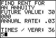 |
This screen shows that we have entered the first three values of the problem: the desired future value, the annual rate, and the number of times per year. | ||||||||||||||||||||||||||||||
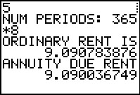 |
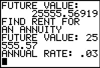
The final bit of data is the number of periods, this corresponding to 8 years with
deposits every day of the year. With all of the data the program computes the required
rent payment if the deposit is at the end of each day (9.090783876) or if it is made
at the start of each day (9.090036749).
[Jump to Figure 56 to see the same
annuity DUE answer from the TVM Solver.]
[Jump to Figure 58 to see the same
ORDINARY annuity answer from the TVM Solver.]
In short, if you can find someone who will pay 3%
on an annuity where you deposit $9.10 each and every day for the next 8 years, that
annuity will be worth over $30,000 at the end of that time.
Return to description table. | ||||||||||||||||||||||||||||||
 |
We will do the LOAN AMOUNT (loan payment determination) twice. First we will follow the description given above. We will find the future value of the amount of the loan at the same interest rate and the same compounding period. Figure 26 indicates that we will use the COMPOUND feature to do this. | ||||||||||||||||||||||||||||||
 |
Most of the data is entered here. | ||||||||||||||||||||||||||||||
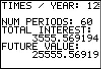 |
After entering the number of periods the program tells us that the original $22,000 would be worth $25,555.57 after the 6 years of monthly compounding at 3%. [Jump to Figure 60 to see the same intermediate answer from the TVM Solver.] Therefore, the next part of the process must determine the rent one would have to pay on an annuity for 6 years, monthly, at 3% to yield the same future value. | ||||||||||||||||||||||||||||||
 |
To do that we return to the RENT FIND option on the second menu. | ||||||||||||||||||||||||||||||
 |
We enter the values. Notice that we have entered the FUTURE VALUE as the rounded $25,555.57. | ||||||||||||||||||||||||||||||
 |
We finish entering the values and the program gives us the option of two answers, one for an ORDINARY annuity and one for an ANNUITY DUE. Assuming that the loan is to be paid back in the usual method, paying at the end of each month, the required loan payment will be $395.32, from the ORDINARY RENT, which has been rounded up so that the payments are complete with the final payment being reduced so that we do not overpay the loan. [Jump to Figure 62 to see the same answer from the TVM Solver.] | ||||||||||||||||||||||||||||||
 |
Of course, it seems strange that we have to do one calculation and then enter the results of that, along with re-entering three of the original variables, in order to get an answer. We should be able to have the program do that for us. And, indeed it will do that. The desired option is the LOAN AMOUNT option, #4. | ||||||||||||||||||||||||||||||
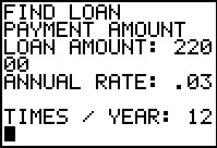 |
This time we enter the original data. | ||||||||||||||||||||||||||||||
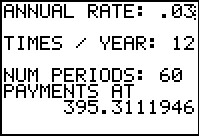 |
And the program just produces the final answer, although it assumes the common
practice of having payments at the end of each period. Thus,
the answer is the same as the value found from an ORDINARY annuity
on Figure 31.
[Jump to Figure 62g to see the same
one step answer from the TVM Solver.]
Return to description table. | ||||||||||||||||||||||||||||||
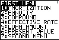 |
Finally, the program does the computations for producing an amortization table. The menu option is the first one: AMMORTIZATION. | ||||||||||||||||||||||||||||||
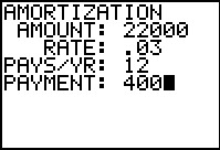 |
The program asks for the required values. | ||||||||||||||||||||||||||||||
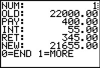 |
Then the program produces the values needed for the first line of the table.
 . .
| ||||||||||||||||||||||||||||||
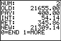 |
The program responds with the data for the second line of the table.
| ||||||||||||||||||||||||||||||
 |
And, the third line...
| ||||||||||||||||||||||||||||||
 |
And, the fourth line...
 key.
That will take us back to the menu system and from there we can get
to the second menu where we can choose the QUIT option. key.
That will take us back to the menu system and from there we can get
to the second menu where we can choose the QUIT option.
Return to description table. | ||||||||||||||||||||||||||||||
 |
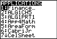
In order to get to the screen shown in Figure 41, press the
 key. The image in this figure was captured
from a TI-84 Plus that had lots of applications installed on it. The
Finance application is the first one listed. It will be the first on on a
TI-83 Plus. We are only interested in the Finance application.
Since it is the highlighted appication, press the key
to start it. key. The image in this figure was captured
from a TI-84 Plus that had lots of applications installed on it. The
Finance application is the first one listed. It will be the first on on a
TI-83 Plus. We are only interested in the Finance application.
Since it is the highlighted appication, press the key
to start it.
| ||||||||||||||||||||||||||||||
 |
The main screen of the Finance application is shown in Figure 42.
At his point we want to use the TVM Solver. That is the highlighted choice so
press the key to start it.
| ||||||||||||||||||||||||||||||
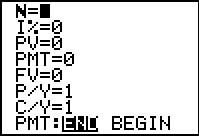 |
Figure 43 has a blank TVM Solver screen. The meanings of the various fields is given by
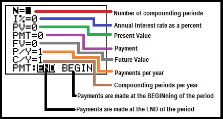  key sequence. We will see this as we solve
the first problem in the next screens. key sequence. We will see this as we solve
the first problem in the next screens.
Return to description table. | ||||||||||||||||||||||||||||||
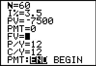 |
For the first problem we set the Present Value to be -7500. It is negative because
TVM Solver looks at the flow of money with negative values meaning you are giving up the
money. If we are investing $7,500 we are giving up control of that money
for the duration of the investment. Therefore, we enter it as a negative value.
The interest is input as a percent, 3.5; the Payment is left as 0 since we are not making any regular
payments. The problem states monthly compounding, therefore we set P/Y to 12 and that will automatically
set C/Y to 12. Then we set the number of periods to 60. Finally,
we move the cursor to the Futurre Value field since this is the unknown.
To have TVM Solver do its work, we press the
key sequence.
The result is shown in Figure 45.
| ||||||||||||||||||||||||||||||
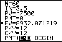 |
The result of our actions in Figure 44 is shown here, the future
value is 8932.071219, a positive value since this is money coming back to us.
The calculator has left a black square next to the Future Value field to indicate that it just solved
for that value.
[Jump to Figure 7 to see the same answer from the FINANCL program.]
Return to description table. | ||||||||||||||||||||||||||||||
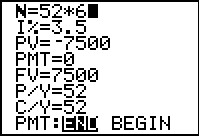 |
In Figure 46 we are setting up the second problem where we want to find the present value. We have set the future value to be 7500 as given in the problem. We also need to enter the number of compounding periods. We will do this by entering the expression 52*6, letting the calculator do the work. | ||||||||||||||||||||||||||||||
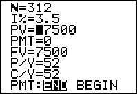 |
Note that the calculator converted our expression of 52*6 to the 312 value.
We have also moved the cursor to the Present Value field since this
is the unknown value for this problem.
Again, we press the
key sequence.
| ||||||||||||||||||||||||||||||
 |
The answer, -6079.811316, is displayed.
[Jump to Figure 12 to see the same answer from the FINANCL program.]
It is negative since this is money
that we would have to commit in order to recieve the 7500 at the end of the
time period.
Return to description table. | ||||||||||||||||||||||||||||||
 |
The third problem type is to find the interest rate needed to
take a given present value and have it produce a given future value
over a specific time period with know compounding frequency.
In Figure 48 we have set all of the given fields and we have positioned the
highlight at the unkown field, I%.
Again, note that for the TVM Solver,we enter the present values as a negative because we
would be giving up control of that money. The future value is positive because we
will be getting that money.
We press the
key sequence to move to
Figure 49.
| ||||||||||||||||||||||||||||||
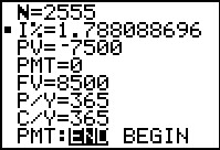 |
The answer is 1.788088696%.
[Jump to Figure 16 to see the same answer from the FINANCL program.]
Return to description table. | ||||||||||||||||||||||||||||||
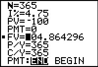 |
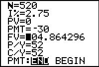
The fourth type of problem is to find the effective rate. There is no direct
field for effective rate within the TVM Solver. However, we can use the
ssystem to get our answer. Figure 50 shows both the setup and the resulot of doing this.
We simply create a convenient present value, $100 (thus setting that field to -100).
Then we set the given annual rate, the frequency
of compounding, and we set the number of periods to correspond to 1 year. Since our
example called for daily compounding we have 365 such periods in the year. Then,
we solve for the Future Value. In this case that came out as 104.864296. But that really
gives us the effective rate since clearly a simple interest rate of 4.864296%
would produce the same result.
[Jump to Figure 19 to see the same answer from the FINANCL program.]
Return to description table. | ||||||||||||||||||||||||||||||
 |
To do an annuity we set the Present Value to 0.
We set the Payment field to -30 representing our deposit of $30 each period.
We set the frequency of payments, in this case 52 to represent weeekly
deposits (the frequency of compounding periods is set to the same value).
We set the number of periods as the number of years times the frequency of periods per year.
We are interested in finding the Future Value so we set the highlight on that field.
Then we press the
key sequence to move to
Figure 52.
| ||||||||||||||||||||||||||||||
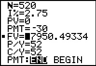 |
Figure 52 gives the answer as 17950.49334 (where the cursor happens to be obscuring
the leading 1 in the screen image).
[Jump to Figure 22 to see the same
ORDINARY annuity answer from the FINANCL program.]
But this is only half of the answer since this
is for an Ordinary Annuity. We know that it is for an Ordinary Annuity
becasue the END at the bottom of the screen is highlighted. In order to get the other half of our answer we will have to change the screen so that the BEGIN becomes highlighted and then we will have to ask for a new computation of the Future Value. | ||||||||||||||||||||||||||||||
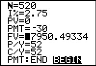 |
To generate the image in Figure 53 we moved the cursor down to the last line and over
to the BEGIN. then we pressed press the
key to switch the highlight to the BEGIN
After that has been done we move the highlight back to the Future Value
field.
That is the state that generated Figure 53. Then we press the
key sequence to move to
Figure 54.
| ||||||||||||||||||||||||||||||
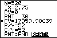 |
Figure 54 gives us the value of the annuity, the Future Value,
for an Annuity Due,
namely, 17959.98639.
[Jump to Figure 22 to see the same
annuity DUE answer from the FINANCL program.]
Return to description table. | ||||||||||||||||||||||||||||||
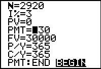 |
In Figure 55 we have set up the next problem, find the required Rent
amount to achieve a given future value. In this case the
Future Value is $30,000, the interest is 3%, payments are to be made daily,
and we still start (Preesent Value) at 0. The highlight has been
placed on the desired value, namely PMT.
Then we press the
key sequence to move to
Figure 56.
| ||||||||||||||||||||||||||||||
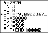 |
The calculator has given us the answer a $9.0900367, but we note that we still have the BEGIN option set at the bottom of the screen. Thus, this the given answer is for a situation where we make deposits at the start of each day. [Jump to Figure 25 to see the same annuity DUE answer from the FINANCL program.] | ||||||||||||||||||||||||||||||
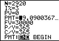 |
The only change in Figure 57 is that we have highlighted the END at the bottom of the screen
and then returned the highlight to the PMT field.
Then we press the
key sequence to move to
Figure 58.
| ||||||||||||||||||||||||||||||
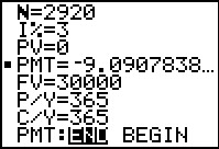 |
Now the answer, corresponding to making deposits at the end of each period,
is given as $9.0907838.
[Jump to Figure 25 to see the same
ORDINARY annuity answer from the FINANCL program.]
Return to description table. | ||||||||||||||||||||||||||||||
 |
As we did using the program above,
we will do the LOAN AMOUNT (loan payment determination) twice.
First we will follow the description given above.
We will find the future value of the amount of the
loan at the same interest rate and the same compounding period.
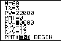
Figure 59 sets up TVM Solver to find the Future value of
us getting $22,00 and holding it for 5 yeears at 3% compounded monthly.
We press the
| ||||||||||||||||||||||||||||||
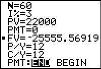 |
We see that we would have to pay back an amount of $25,555.56919 for that loan. [Jump to Figure 28 to see the same intermediate answer from the FINANCL program.] | ||||||||||||||||||||||||||||||
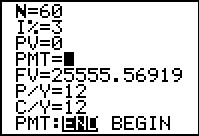 |
In Figure 61 we have changed the Future Value to be positive and we
have set the Present Value to be 0. Now we want to
find the PMT amount that will produce this future value.
We press the
key sequence to move to
Figure 62.
| ||||||||||||||||||||||||||||||
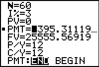 |
Figure 62 shows us that we would have to pay 395.31119 each month to pay off the loan. [Jump to Figure 31 to see the same ORDINARY annuity answer from the FINANCL program.] | ||||||||||||||||||||||||||||||
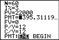 |
As you might expect, the calculator could have done this all in
one step. Figure 62a sets up TVM SOlver to do this.
We have the Present Value set at 22000, the Future Value set at 0,
and the other values stay as before. We will just search directly for the
PMT amount.
We press the
key sequence to move to
Figure 62b.
| ||||||||||||||||||||||||||||||
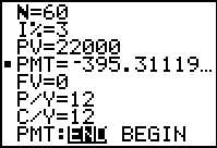 |
Figure 62b shows the same answer, 395.31119 as the payment amount.
[Jump to Figure 34 to see the same
one step answer from the FINANCL program.]
Return to description table. | ||||||||||||||||||||||||||||||
 |
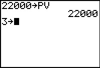
The actions in Figures 63 through 67, with the exception of changing the PMT amount in Figure 67, are redundant since the values of N, P/Y, PV, and PMT have all be set by the previous use of the TVM Solver. However, just for completeness, we could set these outside of that system. For example, to store 22000 into PV we start by creating the screen in Figure 63. | ||||||||||||||||||||||||||||||
 |
To get the PV variable we need to get to the Finance application. | ||||||||||||||||||||||||||||||
 |
Within the Finance application we move to the VARS
screen. Here, as shown in Figure 65, the third item is the PV
variable. We select that option (either by pressing the
 key or by using the
key to move the highlight to item 3
and then pressing the key. key or by using the
key to move the highlight to item 3
and then pressing the key.
| ||||||||||||||||||||||||||||||
 |
Either way, the calculator pastes the PV variable at teh end of the command.
Then we press the to perform the assingment.
In Figure 66 we ccontinue by setting up the command to
store 3 into the I% variable. We would have to return to
the Finance application, and move to the
VARS screen, and select the second item to get that
variable.
| ||||||||||||||||||||||||||||||
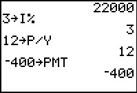 |
Figure 67 shows that we have done all of this. In addition we have set 12 into P/Y and, importantly, we have set the payment to be a nice round $400. | ||||||||||||||||||||||||||||||
 |
Having set those values we can find the remaining balance after n periods by using the built-in function bal(n,d), where n is the number of periods that have completed and d is the number of decimal places to use in our computations. (If d is omitted then the computatiosn are done as per the general calculator settings.) To find the bal( function we return to the main financial application screen and scroll down to item 9, as shown in Figure 68. | ||||||||||||||||||||||||||||||
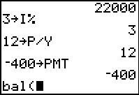 |
Having pasted the bal( symbol onto the screen, we can now complete the command. | ||||||||||||||||||||||||||||||
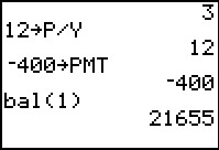 |
In Figure 70 we have completed the command to ask for the balance, without special rounding, after 1 period. The result is the 21655 that we have seen before. | ||||||||||||||||||||||||||||||
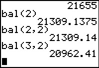 |
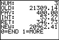
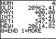
We can recall and repeat the bal( command for other periods of time.
Figure 71 shows this having been done for the
remaining balance after
2 periods, then again after 2 periods but this time rounding to 2 decimal places,
and finally after three periods, again with the 2 decimal place rounding.
[Jump to Figure 40 to see the same
remaining balance answers from the FINANCL program.]
We could, after all, repeat the command for as many periods as we want. We could even build an ammortization table from these results since we know that we are paying $400 each period and by looking at the starting balance for a month and comparing that to the remaining balance at the end of the period, we can see just how much of our $400 went to retire the balance. From that we can compute the amount that went to interest. This becomes a mechanical process for each month so we might code that process into a small program. One such program is AMORTLT and a listing of it si given here: 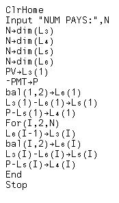 | ||||||||||||||||||||||||||||||
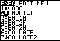 |
To run this program, once it is installed on the calculator, we open the list of programs and select AMORTLT. | ||||||||||||||||||||||||||||||
 |
THis pasts the program name appended to the key phrase prgm onto the screen. Then we run the program. | ||||||||||||||||||||||||||||||
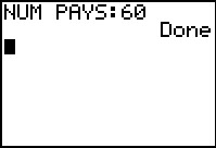 |
The program asks for the number of pays, meaning the number of periods to trace. In Figure 60 we entered this as 60. The program does its work and ends, leaving the results in the various built-in lists. | ||||||||||||||||||||||||||||||
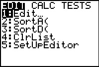 |
To see those lists we take the small precaution of going to the STATmenu and selecting item 5, SetUpEditor. | ||||||||||||||||||||||||||||||
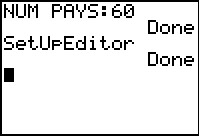 |
The SetUpEditor command was pasted onto the screen and we execute that command. This will make the built-in lists appear in the editor. | ||||||||||||||||||||||||||||||
 |
We return to the STAT menu, this time selecting Edit... | ||||||||||||||||||||||||||||||
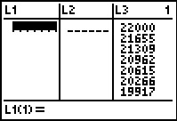 |
Figure 78 shows the first three built-in Lists. Of course, of these we are only interested in L3. | ||||||||||||||||||||||||||||||
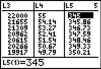 |
We can, however, use the cursors to scroll across to see other lists, as shown in Figure 79. [Jump to Figure 40 to see the same answers from the FINANCL program.] | ||||||||||||||||||||||||||||||
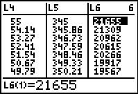 |
And here, in Figure 80 we see the remaining balance list, L6. | ||||||||||||||||||||||||||||||
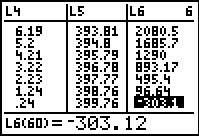 |
In Figure 81 we have moved down the list to the last period where we see that had we paid $400 that last period we would have overpaid by $303.10. Therefore, our final payment would have only been for 96.90. This difference is caused because, back in Figure 67, we set the payment to a nice round $400 instead of trying to come closer to the actual, computed, value $395.31119. In reality, we would have had to have payments of $395.31 (in which case we would have the final payment slightly larger than that to make up the difference), or $395.32 (in which case the final payment would be slightly smaller because we had consistently overpaid). Our choice of $400 was just to make the computations a bit easier. | ||||||||||||||||||||||||||||||
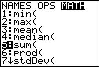 |
One of the more interesting consequences of having the ammortization table built into the lists is that we can use other functions on them. Here we have moved to the LIST menu, then over to the MATH screen, and then down to item 5, sum(. | ||||||||||||||||||||||||||||||
 |
In Figure 83 we see the start of the command pasted onto the screen. | ||||||||||||||||||||||||||||||
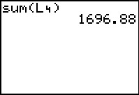 |
We finished the command by placing the list name L4 and the closing parenthesis on the screen. When we execute that command we get the total of the interest paid for the loan. | ||||||||||||||||||||||||||||||
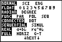 |
Your textbook describes yet another way to achieve the same thing. This method uses the Y= screen to define various functions and the the Finance application to specify those functions. Figure 85 shows the MODE screen. It is presented here just because we want to be sure that the FUNC option is set in the fourth line. | ||||||||||||||||||||||||||||||
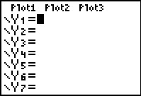 |
Then we move to the Y= screen so that we can define our functions. The first one that we want will hold the interest for a particular period, where the period will be specified by the value of the independent variable X. | ||||||||||||||||||||||||||||||
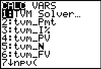 |
To find the desired function we return to the Finance application screen, shown in Figure 87. Our desired function is further on in the list of items on this screen so we will need to scroll down the screen. | ||||||||||||||||||||||||||||||
 |
Figure 88 shows that we have moved down the screen to item A. That is the function for finding the sum of all interest from a starting period through an ending period. We will use this function, placing the value X in both the starting period and ebnding period position so that we can have the calculator compute the interest for month X. | ||||||||||||||||||||||||||||||
 |
Figure 89 shows that we have pasted the desired function onto the screen. | ||||||||||||||||||||||||||||||
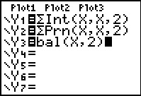 |
Figure 90 not only has the completed statement for the interest function, namely, starting at period X, ending at period X, and rounding results to 2 decimal digits, but also similar functions, also found on the screen in Figure 88, for the amount of the principal retired in period X and the remaining balance at the end of period X. | ||||||||||||||||||||||||||||||
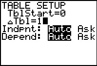 |
Once the functions are set up we move to the TBLSET screen were me have the table start at 0 with step size 1. | ||||||||||||||||||||||||||||||
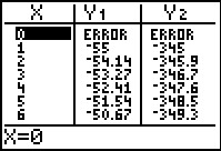 |
From there we move to the TABLE screen where all of our values are shown, at least all the one that fit on the screen. [Jump to Figure 40 to see the same answers from the FINANCL program.] | ||||||||||||||||||||||||||||||
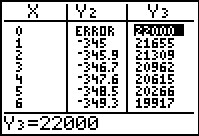 |
Finally, in Figure 93 we have scrolled over to see more of the
values that would go into our amortization table.
Return to description table. | ||||||||||||||||||||||||||||||
©Roger M. Palay
Saline, MI 48176
February, 2012