Chapter 3 Introduction to Detailed Notes

These are notes that I made on my reading of the textbook. There is no real attempt to have comments on absolutely everything in the book noted here. At the same time, there is supplementary material here that is not in the book.

After writing out the notes for the first few sections, it has become clear that there is a tendency to make this a "teaching" document. As much as possible, efforts will be made to not do this. Rather, if there is teaching material to be presented then that will be done in separate pages, with pointers inserted here.

Chapter 3: Polynomial, Rational and Algebraic Functions

Chapter 3, Section 0: Review of Rational Expressions, Rational and Radical Equations

Page 183, in the middle of the division example, change "nextcolumn" to "next column".

Page 184 and following: It is a matter of style, but I prefer to have the terms of the quotient line up with like terms in the dividend. That is, I would have written the first example as:

Note that the TI-89 does this work using its built-in functions and commands and its ability to do symbolic manipulations. The TI-85 and TI-86 do not have this ability. However, there is a program for the TI-85 and TI-86 that will do the multiplication and division of polynomials in one variable. That program is the POLY3 program for the TI-85 amd the POLY3 program for the TI-86. These programs are available on the TI web site.

Even though students can find the correct answer to a polynomial division by using the TI-89 or the POLY3 program on the TI-85 or 86, it might still be nice to be able to generate the entire division problem, with all of the work shown, on the calculator. To this end I have created the polydiv program for the TI-85, the polydiv program for the TI-86, and the polydiv program for the TI-89.

Chapter 3, Section 1: The Remainder, Factor and Root Theorems

This is wonderful material. The Remainder Theorem is a beautiful illustration of just how nicely the pieces of mathematics fit together. Here we have this remarkable result, namely that if we take any polynomial in a single variable, x, and we divide it by the binomial (x-a) where a is some number, then the remainder will be the same value as if we evaluate the original polynomial by replacing x with a. Thus, for

Reloading this page will produce an new example above

Although the beauty of the Remainder Theorem may beam forth from the example(s) above, one might wonder at why it is important at all. First, the Factor Theorem is a direct result of the Remainder Theorem. That is, if the remainder on divison by (x-a) is zero, then we know that (x-a) is a factor of the original polynomial. Second, we really want to find the factors of polynomial so that when we have a problem such as And third, we do not have a nice way to factor the polynomial. However, equiped with the Remainder and Factor Theorems, we can quickly try all sorts of values for a in (x-a). This was especially true before we had calculators and computers that find solutions to problems such as x⁵ – x⁴ – 27x³ + 13x² + 134x – 120 = 0 Here we could easily try solutions such as (x-1) or (x+1) or (x+2) and so forth. We would try them not by doing the division, but rather by applying the Factor Theorem.

Now with an advanced calculator, such as a TI-86, we might use the POLY command to open the screen

where he have indicated that we have a fifth degree polynomial. That produces the screen

where have responded with the appropriate coefficients from the problem. Then we use the SOLVE menu item (F5), to obtain the result shown as

Or, for the TI-89 we need to use the solve() function from the algrbra menu to create the command

which will produce

and, using the cursor keys, we can move to the right to see the rest of the answer line in

In short, these theorems were helpful in testing out possible factors of a polynomial. The Rational Root Theorem is an additional help in that it cuts down the number of values to test as possible roots. That theorem determines a set of possible rational roots. Once we have the list, we can use the Factor Theorem to test those values.

Chapter 3, Section 2: Graphing Polynomial Functions

change the second line to "more difficult to graph than are linear..."

The image at the bottom of page 199 is meant to illustrate end behavior for odd degree cases. Unfortunately, it shows the "middle behavior" at the same time. We do not know what that middle behavior is. It can be quite different for different odd degree cases. A better example might be

where the "middle behavior" is not shown. Note that we do know that we will be below the x-axis at the left of the graph and above it on the right for cases where the leading coefficient is positive. However, we really should not show the y-axis because we do not know, in general, where it is with respect to the graph.

A similar change should be made in the figures at the top and bottom of page 200. A replacement for the first of the Even Degree Case graphs would be

Note that in the general case for even degree polynomials, we are not sure of the location of the x- or the y-axis.

On page 202, change the start of the Turning Points paragraph (note that Turning Points needs to be moved down a line in the book).

The question now arises as to where are the turning points for the graph of f. By inspction of the graph above, we note that there is a turning point between x=^–1 and x=2, and another between x=2 and x=4.

Replace the end of that paragraph with

The precise definition of a relative maximum or minimum will be found in the introductory calculus course. For our purposes we will define them as follows:

The final paragraph on that page starts with "Using a graphics aid..." I believe that the intent here is to suggest using the TRACE feature on the graphics calculator to find the x and y values of points that look like turning points on the graphs.

Descates' Rule of Signs is presented on page 206. We need to recognize that this was a great help in finding roots of a polynomial when we had to do that work by hand. It narrows the search for solutions by telling us the number of possible postive and negaitve roots. Once we have a graphics calculator in hand, we can enter a polynomial and simply look at the places where that polynomial crosses the x-axis.

The presentation of the Fundamental Theorem of Algebra works well. I would emphasize, on page 209 at the end of the first paragraph, the statement "not all necessarily distinct".

Page 210, the last sentence in the section on multiplicity should read "Conversely, a polynomial constructed from complex conjugate roots with integer coefficients will have integer coefficients."

Just above EXAMPLE 14 on page 211, add the statement "However, the grahical approach may not be able to give the precision that we can get with first approach."

As noted earlier in the text, the problem we are looking at is a polynomial inequality in one variable, x. However, to use the calculator we graph the function y=f(x) and then look at the places where the value of the ordinate (the y value) is greater than (or less than) zero. Also, remember that we could just graph the inequality, still using the y= feature, but having the actual inequality on the right side. Thus, with a TI-85 or TI-86, we could plot the function from the top of page 212 by using

y1=(x²+3x–10>0)*4–2 as given in the graph Whereas, the TI-89 (and 92) do not treat the value "true" as 1 and "false" as 0, so we would need to use the function tester(). described earlier in the course, to create y1=tester("x^2+3x–10>0",x)*4–2 which we could graph as

Chapter 3, Section 3: Rational Functions

In version 1 only

Page 218: add a comment on the symbols just above the final section of text that states: The symbols are read "As x approaches positive infinity, 1/x approaches 0".

Page 218: change the last section of text to be "This means that when x is very large, the graph of f(x) is barely different from the graph of y=0.

page 219: change the first section of text to start with "This means that when x is very near to zero, still positive, (but not equal to zero), the graph of f(x) is barely different from the upward portion of the graph of the vertical line x=0.

In version 1 only

The calculator images on pages 220 and 221 have been replaced by new, better graphs in version 2.

It is important to note that I was not able to produce the image on page 223 with the settings that were given there. The image that I was able to produce, given the two functions

y1=(x² – 2x + 3) / ( x – 2)
y2=x with xMin=^–10, xMax=10, yMin=^–10 and yMax=10 is

which is similar to the image in the text, but the image above has the unfortunate almost vertical, connecting line between the left half of the rational function and the right half of that function. That extra line is an artifact of the way that the calculator plots the graph. The calculator will use the xMin and xMax values to determine the values of x that are to be "plugged into" the function. As it turns out, on the TI-86, this means that the calcualtor does not try to use the value x=2. In fact, the calculator moves from x=1.9047619048 (which makes y1=^–29.59523811) to x=2.0634920635 (which makes y1=49.313492058). The calculator is in "DrawLine" mode. Therefore, the calculator tries to connect these two points, producing the near vertical line seen above.

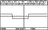
On the other hand, if we shift the calculator to the "DrawDot" mode, we obtain the following graph:

This graph no longer suffers from the addition of the near vertical line, but it does have the limitation that the graph of the rational function "breaks up" near x=2, because the changes in the y values are so dramatic as the value of x gets near to 2. We want to return to the "DrawLine" mode, but we want to set the xMin and xMax values so that the calculator actually evaluates the function for x=2. We can do this by setting xMin=^–12.6 and xMax=12.6. Doing this will cause the calcualtor to try x values in increments of 0.2. The rational function function will eventually be evaluated at x=1.8 (which makes y1=^–13.2), then at x=2 (which the calculator notes makes y1 undefined), and then at x=2.2 (which makes y1=17.2). The graph produced by these settings is:

These graphs illustrate the importance and the impact of changing the WINDOW settings on the graphing calculators.

Page 224; the line at the top does not make sense. Such a rational function does behave like the polynomial portion of the quotient as far as the end-behavior. However, for valus of x where the denominator of the remainder is near zero, that term will significantly change the value of the quoient plus the remainder. That is the region where the rational function does not behave like the polynomial portion of the quotient.

Again, when I try to duplicate the first graph on page 225, I do not get the image given in the text. Rather, I get an image such as

With the indicated settings for the x values, the calculator does not try evaluating the rational function when x is 2. However, changing the WINDOW settings to xMin=^–12.6 and xMax=12.6, produces the graph

because the calculator now does evaluate, or try to evaluate, the rational function when x is 2.

Page 233: The graph has the value -100 in the wrong place. It should be at the left side of the image.

Chapter 3, Section 4: Piece-Wise and Non-Rational Functions

On page 239, it is interesting to note that we can create the entire piece-wise function given at the top of the page within the syntax of the TI-85 and 88 calculators. We merely need to construct the function y1=(x0)*(^–2)+(x0)(x+1) Once again, we are using the fact that the TI-85 and TI-86 treat the value "true" as 1 and the value "false" as 0. The graph of that function is

which looks about right, except for the strange vertical line segment just to the left of the y-axis. This is caused by the calculator being in "DrawLine" mode. If we change to the "DrawDots" mode, the graph becomes

which looks a bit better.

On page 244, about a third of the way down the page, we have the statement

x + 2 0 x ^–2 but we do not have an explanation of the symbol

. That symbol is read "if and only if".

On page 246 the book introduces the "greatest integer function". We actually have that function on the calculator. It is called the "int" function. If we use the function

y1=int(x) we will get the graph

which has the unfortunate vertical connector lines, created because the calculator was in "DrawLine" mode. If we switch to "DrawDots" mode, we get the graph

The real difficulty here is that it is hard to see the "open" versus the "closed" end of the steps.

We can use the greatest integer function in an expression, such as

y1=x–int(x) The graph for that function is given as

The TI calculators have another function, called iPart, that is similar to, but not the same as, the greatest integer function, int. The iPart function produces the integer portion of the the argument (the data being evaluated). Thus,

x	int(x)	iPart(x)
5	5	5
^–5	^–5	^–5
6.2	6	6
^–5.1	^–6	^–5
^–4.96	^–5	^–4

A graph of

y1=iPart(x) is

Note the similarity to the greatest integer function. The difference is that the portion of the graph to the left of the y-axis has been pushed up one step. Of course, we can use the iPart function in an larger function. For example, we can look at the function y1=x–iPart(x) which has a graph that looks like