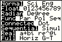
| First we want to be sure that the
calculator has the correct mode settings.
To do this, use
 to display a screen similar to Figure 1.
All of the options on the left,
and only the options on the left, should be highlighted. If your screen does
not appear like this, then you should fix it. Use the cursor control keys to move up and down,
left and right on the screen. Then use the
  key to select the
desired option.
To get out of the review of modes, press the key to select the
desired option.
To get out of the review of modes, press the  . .
|
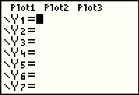
| We will start with Example 1 from the book: Determine whether (a) (2,13) and (b) (-1,-3) lie on the graph of y=10x-7.
To do this we will set the graphing function Y1 to be 10X-7. Press
the  key to open the screen in Figure 1. key to open the screen in Figure 1.
|
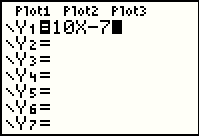 |
We enter the desired function using the
  
  keys.
Then, we can complete the task and move to get a graph
of this line by pressing the keys.
Then, we can complete the task and move to get a graph
of this line by pressing the  key. key.
|
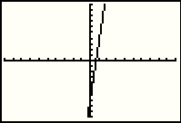 |
Here is a graph of the function y=10x-7 but we cannot really see if the two given points are on the line. |
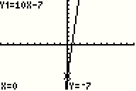 |
The caluclator has a feature that can help us here, namely the TRACE feature. Enter this
by pressing the  key. THis should put the
calculator into the trace mode and
display the modified graph as in Figure 4. Note that there is a blinking (well, not blinking on the
web page but blinking on the screen) cursor on the line. Fruthermore, at the top of the
screen the calculator shows us the particular function being traced, in this case Y1=10X-7.
The coordinates of the point being highlighted appear at the bottom of the
screen so we can see that the cursor is at the point (0,-7). key. THis should put the
calculator into the trace mode and
display the modified graph as in Figure 4. Note that there is a blinking (well, not blinking on the
web page but blinking on the screen) cursor on the line. Fruthermore, at the top of the
screen the calculator shows us the particular function being traced, in this case Y1=10X-7.
The coordinates of the point being highlighted appear at the bottom of the
screen so we can see that the cursor is at the point (0,-7).
|
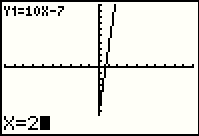 |
We can move that cursor to the point that has its x-coordinate being 2 by
pressing the  key to generate Figure 5, and then pressing the key to generate Figure 5, and then pressing the
 key to move to Figure 6. key to move to Figure 6.
|
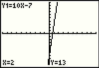 |
The cursor has disappeared in Figure 6 because the point (2,13) is off the screen. However, the calculator has confirmed that the point (2,13) is on the line y=10x-7. |
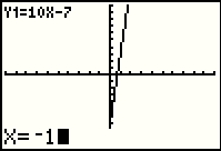 |
To check on the other point (-1,-3), we type   to generate Figure 7. We follow that with
  key to
move to Figure 8. key to
move to Figure 8.
|
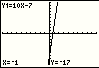 |
Reading the coordinates at the bottom, we see that the point (-1,-17) is on the line. That means that (-1,-3) is not on the line, something we should have noted from inspection of the graph since the line crosses the y-axis at (0,-7) and moves down and to the left from there. (-1,-3) is up and to the left of the y-intercept. |
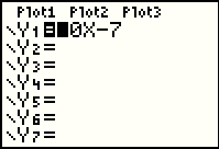 |
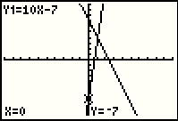
Without losing our original function, we can enter the function of Example 2, namely, y=7-3x,
into the calculator. Press the  key to return to the Y= screen as
shown in Figure 9. Note that the screen capture that produced Figure 9 happened to catch the blinking
cursor as a black rectangle that is covering the 1 of the 10X-7. key to return to the Y= screen as
shown in Figure 9. Note that the screen capture that produced Figure 9 happened to catch the blinking
cursor as a black rectangle that is covering the 1 of the 10X-7.
|
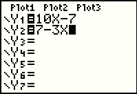 |
To enter the new function use the  key to move to the Y2= line, then
enter the function using the
keys key to move to the Y2= line, then
enter the function using the
keys  
  , producing the image shown in Figure 10. , producing the image shown in Figure 10.
|
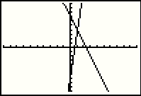 |
Pressing the  key displays the graph of Figure 10a,
with both lines on it. key displays the graph of Figure 10a,
with both lines on it.
|
 |
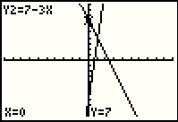
Return to TRACE mode using the  key. Note that the
calculator is again tracing the first function, Y1=10X-7. key. Note that the
calculator is again tracing the first function, Y1=10X-7.
|
 |
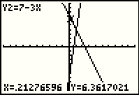
Press the  key to change the trace to the next
function, in this case Y2=7-3X. We see that the cursor is at the point (0,7). key to change the trace to the next
function, in this case Y2=7-3X. We see that the cursor is at the point (0,7).
|
 |
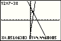
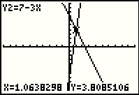
Press the  key to move to the next pixel position to the
right on the graph. The highlight moves a,d the coordinates change. This is the point
(.21276596,6.3617021). That is not a pretty pair of values, but it is on the
line. We might want to find a nicer spot so we can continue to press
the key to move to the next pixel position to the
right on the graph. The highlight moves a,d the coordinates change. This is the point
(.21276596,6.3617021). That is not a pretty pair of values, but it is on the
line. We might want to find a nicer spot so we can continue to press
the  key until we ge the screen shown in Figure 14. key until we ge the screen shown in Figure 14.
|
 |
We are getting close to having the x value be 1. |
 |
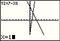
Press the  key one more time and we are at
the display in Figure 15. Here we have moved beyond having x=1. key one more time and we are at
the display in Figure 15. Here we have moved beyond having x=1.
|
 |
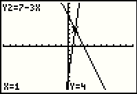
As demonstrated before, we can have the calculator evaluate the function at a
particular point while in the TRACE mode by entering that x value. To get Figure 16 we
press the  key. key.
|
 |
Complete the process by presing the  key.
In FIgure 17 we see that the point (1,4) is on the graph. key.
In FIgure 17 we see that the point (1,4) is on the graph.
|
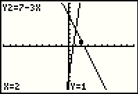 |
To find the coordinates of the point that has the x-coordinate as 2, we
press   . This produces Figure 18
where we find that (2,1) is on the line. . This produces Figure 18
where we find that (2,1) is on the line.
We could enter even more x-values and for each one the calculator will give us the corresponding y-coordinate. We would just have to write down each pair as we generate it. Perhaps there are other ways to generate such lists of values. |
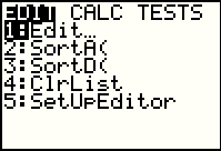 |
One way to do this is to generate a list of x values and then compute the
corresponding list of y values. Press the  key to open the
screen shown in Figure 19. As it opens the first option, Edit, is highlighted.
Press the key to open the
screen shown in Figure 19. As it opens the first option, Edit, is highlighted.
Press the  key to move to Figure 20 where we can edit the lists. key to move to Figure 20 where we can edit the lists.
|
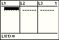 |
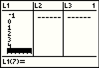
Figure 20 shows the screen as it will appear if there are no values already in the L1, L2, and L3 lists. The screen also shows that the calculator is waiting for us to give it a value to put as the first item in L1. |
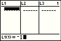 |
Press   to indicate
that we want that first item to be -1. to indicate
that we want that first item to be -1.
|
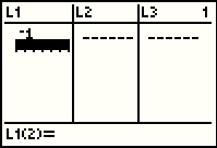 |
Complete the entry by pressing the  key. The -1 appears in
L1 and the calculator is ready to accept
a value for the second item in L1. key. The -1 appears in
L1 and the calculator is ready to accept
a value for the second item in L1.
|
 |
We enter the rest of the values by pressing


  in order to produce Figure 23.
|
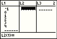 |
At this point we press the  key to move to the second
column, L2. key to move to the second
column, L2.
|
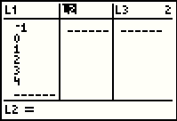 |
We want to have the calculator compute values for L2. We use the
 key to move the highlight out of the list items and onto the list name, L2.
Note that at the bottom of the screen the calculator now asks for a definition of L2. key to move the highlight out of the list items and onto the list name, L2.
Note that at the bottom of the screen the calculator now asks for a definition of L2.
|
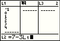 |
for Figure 26 we have entered the desired expression by using the
  
  key sequence. Note that we are nomaking reference to the definition in Y2.
Rather we are entering the expression again, this time using L1. key sequence. Note that we are nomaking reference to the definition in Y2.
Rather we are entering the expression again, this time using L1.
|
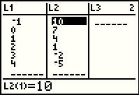 |
We press  to move to Figure 27 where the values of
L2 have been computed and displayed. Here, in one screen, we have all the values that we need
for Example 2. to move to Figure 27 where the values of
L2 have been computed and displayed. Here, in one screen, we have all the values that we need
for Example 2.
There is a problem with this, however. The values have been computed and are no
longer tied to either the value in L1 nor to the definition that
we entered. To see this we start by pressing
|
 |
We can demonstrate the problem by changing one of the values in the first column. The first value is highlighted so we might as well change that one. |
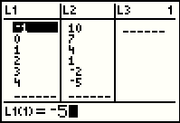 |
Press the   kys to
enter -5 at the bottom. To move to Figure 30, press the kys to
enter -5 at the bottom. To move to Figure 30, press the  key.
key.
|
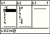 |
Note in Figure 30 that the first value in the L1 list has indeed changed, but that such a change had no effect on the corresponding value in the second column. |
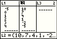 |
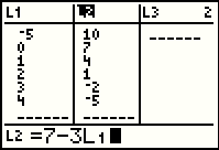
To start to correct this we use the  key
to move to the second column and then the key
to move to the second column and then the 
 sequence to put the highlight at the heading of the second column, L2.
Note that the bottom of the display shows the definition of L2. It is no longer the 7-3L1
that we entered in Figure 26. It is now just the list of values. sequence to put the highlight at the heading of the second column, L2.
Note that the bottom of the display shows the definition of L2. It is no longer the 7-3L1
that we entered in Figure 26. It is now just the list of values.
|
 |
We replace that list of values with a retyping of the definition, 7-3L1. |
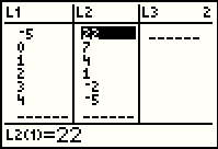 |
Press  to produce Figure 33. Again, at this point the values
in the two lists represent the coordinates of points on the line. to produce Figure 33. Again, at this point the values
in the two lists represent the coordinates of points on the line.
|
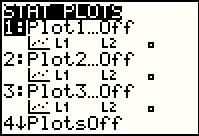 |
We can actually plot the points identified in Figure 33. To do this we need to be sure that the
calculator is set to plot points where the x-coordinate is in L1 and the y-coordinate is in L2.
We press the   keys to
open the STAT PLOTS screen shown in Figure 34. The first of the
STAT PLOTS is highlighted and it shows that Plot1 is Off and that
Plot1 is already set to plot points using L1 and L2.
Because it is currently selected, to get to the detail of Plot1 we press the keys to
open the STAT PLOTS screen shown in Figure 34. The first of the
STAT PLOTS is highlighted and it shows that Plot1 is Off and that
Plot1 is already set to plot points using L1 and L2.
Because it is currently selected, to get to the detail of Plot1 we press the
 key. key.
|
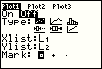 |
Figure 35 shows the screen as we have moved to the details of Plot1, with the exception that you cannot see the
blinking cursor. IT happens to be on the ON option. To select the option
press the  key. That will move us to Figure 36.
highlighted key. That will move us to Figure 36.
highlighted
|
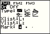 |
Now the ON option is selected. The blinking cursor is still on that option.
We can finally move to the graph by pressing the  key. key.
|
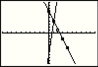 |
Figure 37 is similar to Figure 10a, but with the addition of the points we have plotted. You might note that out first point, from Figure 33, (-5,22), is not shown because it is off the displayed window of the graph. |
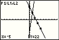 |
To get to Figure 38 we press the
 key to move back to the TRACE feature of the
calculator. When we did this before, in Figure 4 and Figure 11, the calculator
started the TRACE looking at the first function, Y1=. This time it
has started the trace looking at Plot1 represented in the upper left
corner of the screen by P1:L1,L2.
Within that Plot1, the trace starts with the point at X=-5 and Y=22, which,
as noted above, is off the screen. THese values are given at the bottom of the screen. key to move back to the TRACE feature of the
calculator. When we did this before, in Figure 4 and Figure 11, the calculator
started the TRACE looking at the first function, Y1=. This time it
has started the trace looking at Plot1 represented in the upper left
corner of the screen by P1:L1,L2.
Within that Plot1, the trace starts with the point at X=-5 and Y=22, which,
as noted above, is off the screen. THese values are given at the bottom of the screen.
|
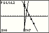 |
Press the  to move to the next point of Plot1,
namely (0,7). Note how the values change at the bottom of the screen, and, since that point
is on the screen, there is now a flashing highlight on that point. to move to the next point of Plot1,
namely (0,7). Note how the values change at the bottom of the screen, and, since that point
is on the screen, there is now a flashing highlight on that point.
|
 |
The fact that we are missing one of our plotted points is a little inconvenient.
THe TI-83 provides a feature to change the window so that all of our plotted
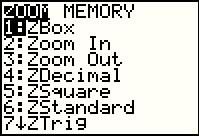
points will be on the screen. We press the
 key to open the ZOOM window in Figure 40. key to open the ZOOM window in Figure 40.
|
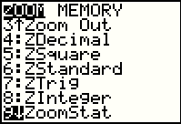 |
The option that we want, ZoomStat, is not displayed in Figure 40, so we use the
down cursor button,  , to move the highlight down to option 9
as shown in Figure 41. , to move the highlight down to option 9
as shown in Figure 41.
Then, press the |
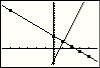 |
Having changed the window by using the ZoomStat feature in Figure 41, the
calculator redisplays the plots and graphs, but this time with the window
settings such that all of the Plot1
points are displayed on the screen. A consequence of the previous action is that the graph looks different in that the lines are not nearly as steep as they were before. The reason for this is that the range4 of the y-axis has been increased dramatically to allow for the point (-5,22). That compresses the y-axis, effectively squishing down the graph to fit into the window. |
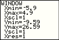 |
We can look at the WINDOW settings by pressing the  key.
The settings in Figure 42 are the result of our earlier action of using the ZoomStat feature.
Note that the x values are spread actross the wide part of the screen from -5.9 to 4.9.
The y values are spread across the narrow part of the screen from -9.59 to 26.59. key.
The settings in Figure 42 are the result of our earlier action of using the ZoomStat feature.
Note that the x values are spread actross the wide part of the screen from -5.9 to 4.9.
The y values are spread across the narrow part of the screen from -9.59 to 26.59.
|
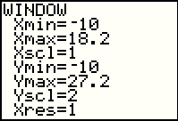 |
Of course, we can change these values. We do this by using the cursor keys to move through the fields and we
enter new values as we see fit. One thing to keep in
mind as we do this is the actual number of pixels (picture elements, the dots that make up the screen)
on the calculator. There are 95 horizontal pixels across the calculator and 63 vertical
pixels from top to bottom on the display. We could number the pixels
from 0 to 94 across and 0 to 62 up and down.
The 94 and 62 values are important to remember.
[For a more in depth look at pixels on the TI-83 see the Pixels on TI-83
page.]
Thus, if we choose a span on the x values that is some multiple of 94 then we will have some nice
even steps across the screen. In this case, in Figure 44, we have selected -10 as
the Xmin value and
set 18.2 as the Xmax value. Thus, the horizontal spread is 28.2 or 3*94/10.
As we will see,
each step across the screen will represent a change of 3/10 or 0.3 unitls. The Ymin is set as -10 and Ymax is set to 27.2. This represents a spread of 37.2 or 6*62/10. As such each step up and down on the screen will represent a change of 6/10 or 0.6 units. The Yscl value was changed to 2 so that the tick marks on the y-axis area spread out a bit. We see in Figure 42 that these tick marks pile up on each other. |
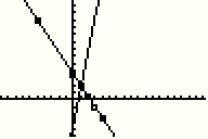 |
Press the  key to return to the graph, this time with
new WINDOW settings. All of the points are still here and again the slope of the lines has changed.
We might note that the changes that we made in Figure 44 represent little change in the
spread of the y values from what they
were in Figure 43. However, the spread of the x values has increased significantly. Thus
we are squeezing more x values onto the screen. In effect, we are squeezing the screen
horizontally, thus making the lines look steeper. key to return to the graph, this time with
new WINDOW settings. All of the points are still here and again the slope of the lines has changed.
We might note that the changes that we made in Figure 44 represent little change in the
spread of the y values from what they
were in Figure 43. However, the spread of the x values has increased significantly. Thus
we are squeezing more x values onto the screen. In effect, we are squeezing the screen
horizontally, thus making the lines look steeper.Also note the nice spread of the tick marks on the y-axis because of the change that we made to the Yscl value. |
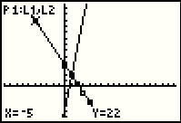 |
For Figure 46 we turn on the TRACE feature by using the  key.
As expected the TRACE feature again starts with the Plot1 values. key.
As expected the TRACE feature again starts with the Plot1 values.
|
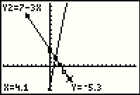 |
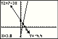
Remember that the up and down cursors are used to move from one plot ot graph to the next.
Pressing the  will take the TRACE to
the graph before the Plot1,
namely, Y2=7-3X. Note the nice values that we hit. Such nice values are the consequence
of our choices for the Xmin, Xmax, Ymin, and Ymax values. will take the TRACE to
the graph before the Plot1,
namely, Y2=7-3X. Note the nice values that we hit. Such nice values are the consequence
of our choices for the Xmin, Xmax, Ymin, and Ymax values.
|
 |
Pressing the  key once moves us to a different point and,
as anticipated, the x value has dropped by 0.3 units. key once moves us to a different point and,
as anticipated, the x value has dropped by 0.3 units.
|
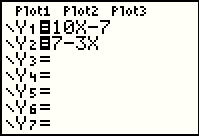 |
There is yet another way that we can use the TI-83 to help with Example 2. First,
we return, in Figure 48a, to the Y= screen by pressing the
 key.
We see our definitions for Y1 and Y2 here. key.
We see our definitions for Y1 and Y2 here.
|
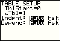 |
Then we want to look at the TBL SET screen, so we press the
  keys to get Figure 48b. The settings
shown here mean that when we move to the TABLE screen the independent vaiable, X,
will start with a value of 0, it will increase by 1 for each row of the table,
and that the values of the independent variable and the dependent variable
will automatically be displayed. keys to get Figure 48b. The settings
shown here mean that when we move to the TABLE screen the independent vaiable, X,
will start with a value of 0, it will increase by 1 for each row of the table,
and that the values of the independent variable and the dependent variable
will automatically be displayed.
|
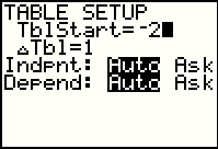 |
For illustration, we will set the TblStart value to -2. Then, press the
  keys to move to the
TABLE screen, shown in Figure 48d. keys to move to the
TABLE screen, shown in Figure 48d.
|
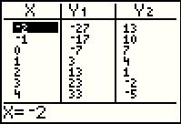 |
In this image we see that the TI-83 has created a table of values for X, Y1, and Y2. The X values, as the independent variable, start at -2 and increase by 1 with each row. The values in the Y1 column are calculated based upon the function definition for Y1 that we saw in Figure 48a. The values in the Y2 column are calculated based upon the function definition for Y2 that we saw in Figure 48a. Thus, in just a few steps, we have lots of values for the coordinates of points on the two functions that we have been using. |
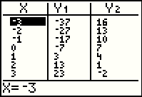 |
Because all of this is automatic, we can use the cursor key to move up the table.
Press  to move up one row. Note that the new values for all three variables are automatically
computed. to move up one row. Note that the new values for all three variables are automatically
computed.
|
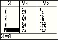 |
Naturally, we could use the  key to move down the list. If we do this a
number of times we can get to the row for X=8 as shown in Figure 48f. Note also that
in Figure 48 the first X value is 2. key to move down the list. If we do this a
number of times we can get to the row for X=8 as shown in Figure 48f. Note also that
in Figure 48 the first X value is 2.
|
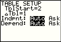 |
Pressing   to return to the
TBL SET screen in Figure 48g, we see that by changing the screen in Figure 48f as we did
the calculator has changed the TBL SET settings to have the TblStart
value now be 2. to return to the
TBL SET screen in Figure 48g, we see that by changing the screen in Figure 48f as we did
the calculator has changed the TBL SET settings to have the TblStart
value now be 2.
|
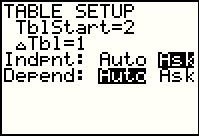 |
To get to Figure 48h we bring the blinking cusor down to the
Indpnt line and move it over the Ask
option, and then press the  key.
In this mode the calculator will ask us for values for the independent
variable, X.
|
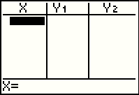 |
Returning to the TABLE screen via the
  key sequence,
we see in Figure 48i that the values are no longer generated by the TI-83.
Instead, the TI-83 is waiting for us to enter the desired values for the independent variable. key sequence,
we see in Figure 48i that the values are no longer generated by the TI-83.
Instead, the TI-83 is waiting for us to enter the desired values for the independent variable.
|
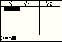 |
If we press the  key the calculator display esponds as in
Figure 48j. key the calculator display esponds as in
Figure 48j.
|
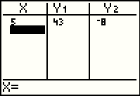 |
Pressing the  key moves the calculator display to Figure 48k.
Now the value 5 has been added to the table and the corresponding values for Y1
and Y2
have been added to the table.
These values have been comuted using the definitions of Y1 and Y2 that we saw
in Figure 48a in the Y= screen. key moves the calculator display to Figure 48k.
Now the value 5 has been added to the table and the corresponding values for Y1
and Y2
have been added to the table.
These values have been comuted using the definitions of Y1 and Y2 that we saw
in Figure 48a in the Y= screen.
|
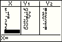 |
To demonstrate a bit more of the TABLE feature,
Figure 48l shows the results of adding new values to the X
column of the table, namely, -1, -6, 3, 4, and 5. Since
we decide the values for the X column there
is no particular order or spacing of the values
and values can be repeated. For each value in the X
column, the TI-83 computes the corresponding value in the Y1 and Y2 columns.
The automatic feature, and the fact that we are using the definitions of Y1 and Y2 for our computations, is an advantage over the use of L1, L2, STAT -- EDIT, and STAT PLOT demonstrated above. The disadvantage of using the TABLE approach is that we cannot graph the TABLE points automatically. |
 |
To move away from Examples 1 and 2 and onto Example 3, we should really turn off the
exisiting plot and then enter a new definition for the new function of Example 3.
Press |
 |
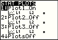
This is the current setting of Plot1. |
 |
Move the highlight to the Off option and then press  to make Off the chosen option.
|
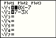 |
Press the  key to move to the Y= screen, shown in Figure 52. key to move to the Y= screen, shown in Figure 52.
|
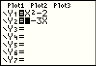 |
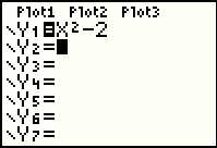
Press the  
 
  keys to get to Figure 53.
Note that the DEL key was needed because we still had the 7 left on the line from
the earlier value. keys to get to Figure 53.
Note that the DEL key was needed because we still had the 7 left on the line from
the earlier value.
|
 |
Pressing the  key deletes the entire definition of Y2 in
Figure 54. key deletes the entire definition of Y2 in
Figure 54.
|
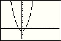 |
Now we are ready to graph the function. Press the
 key to do so. The result is shown in Figure 55. key to do so. The result is shown in Figure 55.
|
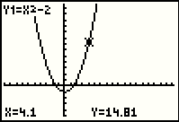 |
We go to the TRACE feature by pressing the  key.
You might note that the X value selected was 4.1, the same initial X value that we found in
Figure 47. This is due to the fact that we have not changed the WINDOW settings that we last saw
in Figure 44. key.
You might note that the X value selected was 4.1, the same initial X value that we found in
Figure 47. This is due to the fact that we have not changed the WINDOW settings that we last saw
in Figure 44.
|
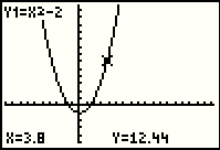 |
Indeed, if we press the  key
we see the highlight move to the X=3.8 value, just
as in Figure 48. key
we see the highlight move to the X=3.8 value, just
as in Figure 48.
|
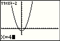 |
Although moving the cursor left and right gives us nice values for X, we are moving
in steps of 0.3. From 4.1 we are not going to get to the value of 4 in
that way.
Fortunately, we can still just press the  key to enter that value, as
in Figure 58. key to enter that value, as
in Figure 58.
|
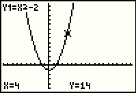 |
Press the  key and the TRACE feature responds by giving
Y=14 and highlighting the point holding (4,14) on the curve. key and the TRACE feature responds by giving
Y=14 and highlighting the point holding (4,14) on the curve.
|
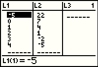 |
Our values in L1 and L2 have not changed. We press
  to move to and through the STAT screen
and arrive at Figure 60. to move to and through the STAT screen
and arrive at Figure 60.
|
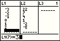 |
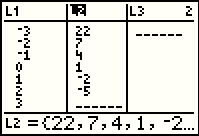
For Figure 61 we have changed the values stored in L1 |
 |
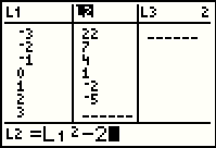
For Figure 62 we have used the  key to
move to the L2 column and then the key to
move to the L2 column and then the  key, repeatedly, to
move the highlight to the heading L2. key, repeatedly, to
move the highlight to the heading L2.
|
 |
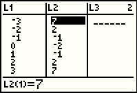
In Figure 63 we have entered the expression for our function, subsituting L1 for X.
The key strokes for this are
 
   . .
|
 |
To move to Figure 64, press the  key and
the TI-83 computes and displays the new values for L2. key and
the TI-83 computes and displays the new values for L2.
|
©Roger M. Palay
Saline, MI 48176
August, 2010