Worksheet 03.4: Descriptive Measures Again

Return to Topics page
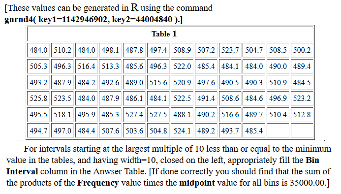
The task here is to come up with descriptive measures for the data in Table 1.

This page assumes that you have read through earlier pages and that you have mastered the steps that we use to set up our work. To that end we will assume that we have

inserted our USB drive,
created a directory called worksheet034 on that drive
have copied model.R from our root folder into our new folder,
have renamed that new copy of the file to the name ws34.R, and
have double clicked on that file to open RStudio.

The result should be a window pretty much identical to the one shown in Figure 1. {Recall that the images shown here may have been reduced to make a printed version of this page a bit shorter than it woud otherwise appear. In most cases your browser should allow you to right click on an image and then select the option to View Image in order to see the image in its original form.}

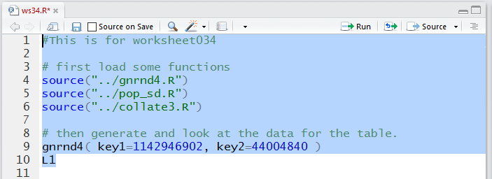
Figure 1

Much of the discussion that would be given here has been included in the comments in our ws34.R file. Therefore, it is important to read those comments. We start by loading the various functions we will need. Then we generate the data values and examine them to be sure that we have the correct values.

Figure 2

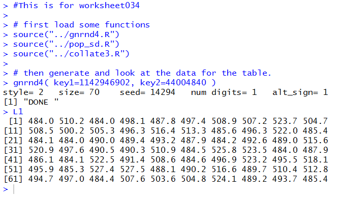
The console view of those commands:

Figure 3

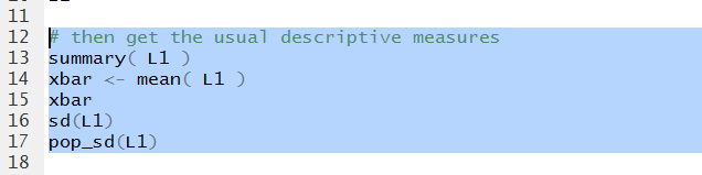
The we add the commands to generate many of our descriptive statistics.

Figure 4

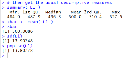
In Figure 5 we can see all of those values.

Figure 5

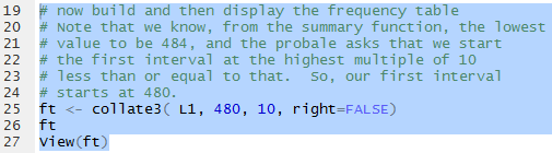
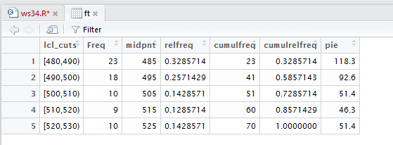
Now we want to generate the frequency table. We are given specific direction on the start of the first bin and the width of the bins. Note that we are storing the generated table in the variable ft, then displaying that table in the Console pane, then displaying it in a better format via the View(ft) command.

Figure 6

In Figure 7 we can read the frequency table values in the Console pane.

Figure 7

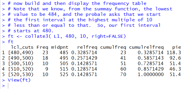
Figure 8 shows the same values, but in a more fancy display.

Figure 8

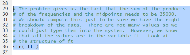
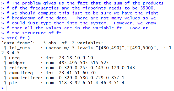
As stated in the comment shown in Figure 9, we really could just re-enter the five values for the frequencies and the five vales for the midpoints. However, since they are already in the system, after all we did see them in the table, we can go look for them. The command str(ft) has R display the structure of the data frame called ft.

Figure 9

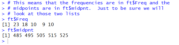
In Figure 10 we note that the frequency values are stored in ft$Freq while the midpoint values are stored in ft$midpnt.

Figure 10

We use those two names just to prove to ourselves that they hold the values that we need.

Figure 11

A run of those commands gives the output shown in Figure 12.

Figure 12

That is good enough for us so we can use the two variables to generate our desired sum.

Figure 13

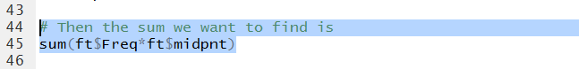
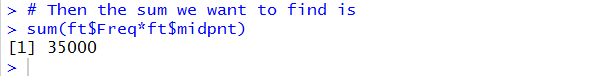
Figure 14 shows the resulting computed value. It checks with the value given in the problem so we feel confident that we have done the right thing.

Figure 14

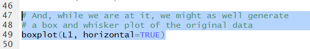
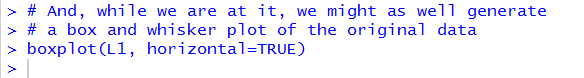
In Figure 15 we form the command to generate a bax and whisker plot.

Figure 15

Running that command does not provide much in the Console pane, shown in Figure 16.

Figure 16

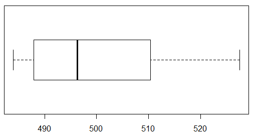
However, in the Plot pane we find quite an acceptable chart.

Figure 17

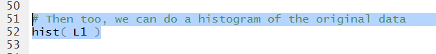
The hist(L1) command will produce a default histogram.

Figure 18

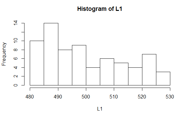
That histogram appears in the Plot pane as shown in Figure 19.

Figure 19

All that is left to do is to save our ws24.R file and then type the q() command in the Console, respond to the prompt with y, and press the Enter key to close our RStudio session.

Figure 20

Here is a listing of the complete contents of the ws34.R file:

#This is for worksheet034

# first load some functions
source("../gnrnd4.R")
source("../pop_sd.R")
source("../collate3.R")

# then generate and look at the data for the table.
gnrnd4( key1=1142946902, key2=44004840 )
L1

# then get the usual descriptive measures
summary( L1 )
xbar <- mean( L1 )
xbar
sd(L1)
pop_sd(L1)

# now build and then display the frequency table
# Note that we know, from the summary function, the lowest
# value to be 484, and the problem asks that we start
# the first interval at the highest multiple of 10
# less than or equal to that.  So, our first interval 
# starts at 480.
ft <- collate3( L1, 480, 10, right=FALSE)
ft
View(ft)

# The problem gives us the fact that the sum of the products
# of the frequencies and the midpoints needs to be 35000.  
# We should compute this just to be sure we have the right
# breakdown of the data.  There are not many values so we
# could just type them into the system.  However, we know 
# that all the values are in the variable ft.  Look at
# the structure of ft
str( ft )

# This means that the frequencies are in ft$Freq and the
# midpoints are in ft$midpnt.  Just to be sure we will 
# look at those two lists
ft$Freq
ft$midpnt

# Then the sum we want to find is
sum(ft$Freq*ft$midpnt)

# And, while we are at it, we might as well generate
# a box and whisker plot of the original data
boxplot(L1, horizontal=TRUE)

# Then too, we can do a histogram of the original data
hist( L1 )