Central Tendency Worksheet (Mac USB Version)
Return to Topics page
Find the mean, median, and mode values for each of the following
four sets of data.
To do this work we will employ the same strategy that we have used
in earlier examples:
- Insert the USB drive
- Create a new folder (directory) to hold our work
- Copy copy our
model.R file
to the new directory
- Rename the new file
- Start RStudio by double clickng on the new file
- Put the desired commands into the editor pane
- Save that that work in the file
- Perform the commands by highlighting the commands
that we want to run, then pressing the
Run icon.
- Observe the results in the Console pane
- Finally, close RStudio
- Safely remove the USB drive
Let us start the process.
Insert the USB drive. This, after a moment or two, opens the
 icon on the desktop.
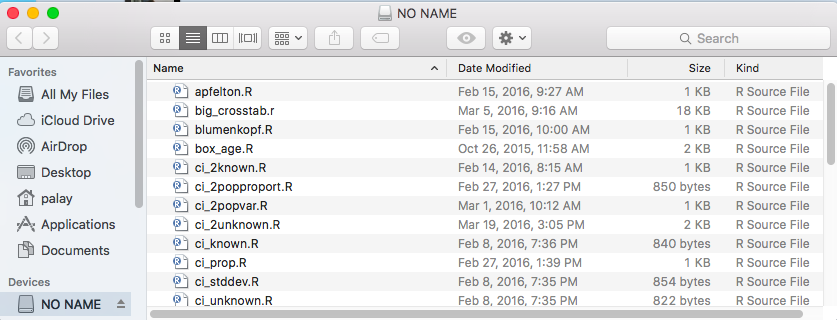
If we click on that we
cause the Finder
to open a window such as the one shown in Figure 1.
icon on the desktop.
If we click on that we
cause the Finder
to open a window such as the one shown in Figure 1.
Figure 1
Click on the Finder menu option File
to open the window shown in Figure 1.5.
Figure 1.5
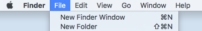
Click on the New Folder option to get Figure 2.
Figure 2
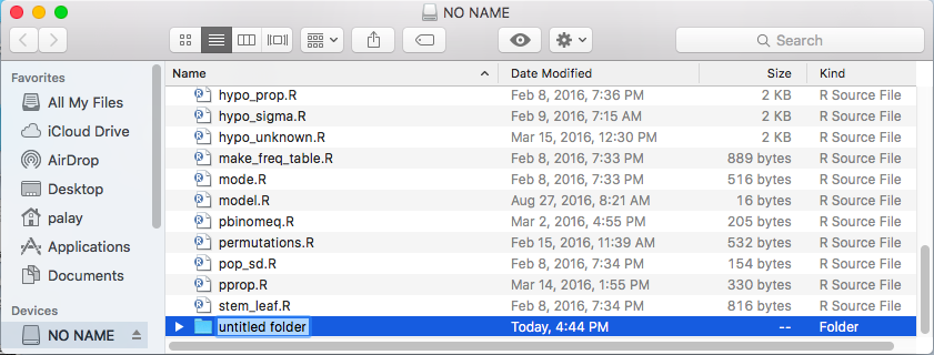
Rather than use the default folder name, Nuntitled folder
of Figure 2, type in a new name. For this project I used
 .
.
Once the folder has been created and renamed, we locate the model.R
file in the list, point to it and right click to open the window
shown in Figure 3.
Figure 3
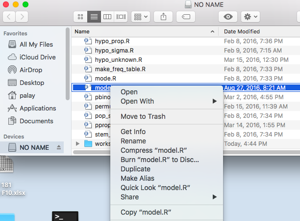
In that window we select the Copy "model.R" option.
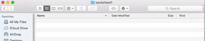
After that we return to find our worksheet1 directory and
we double click on it to open the newly
created empty directory shown in Figure 4.
Figure 4
Then point to an open area, right click, and you should see the
small window in Figure 5.
Figure 5
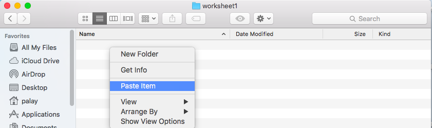
There you want to select the Paste option
to get the copy of the file put into our new directory.
We can rename the file (click on it once, wait a second, and click again
to highlight the name of the file) as shown in Figure 6.
Figure 6
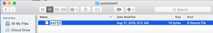
We ctype the new name, ws01.R
as shown in Figure 7.
Figure 7
Once that is in place we can double click on the new file name
to open RStudio, shown in Figure 8.
Figure 8
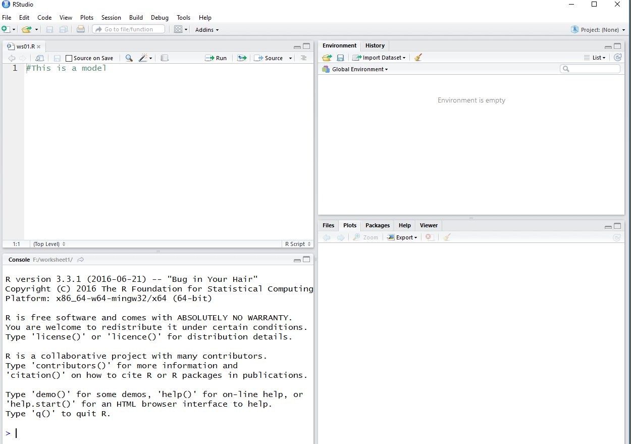
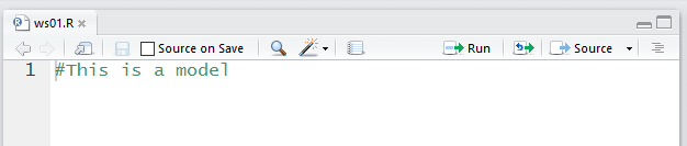
A closer examination of the Editor pane is shown in
Figure 9. This is just what we expect since
we know this to be the contents of the original modl.R
file.
Figure 9
However, we want different commands.
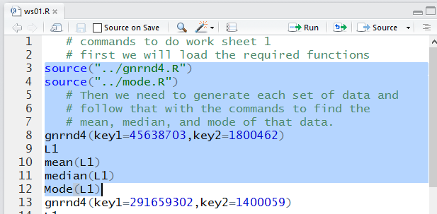
The commands that we want are:
   # commands to do work sheet 1
   # first we will load the required functions
source("../gnrnd4.R")
source("../mode.R")
   # Then we need to generate each set of data and
   # follow that with the commands to find the
   # mean, median, and mode of that data.
gnrnd4(key1=45638703,key2=1800462)
L1
mean(L1)
median(L1)
Mode(L1)
gnrnd4(key1=291659302,key2=1400059)
L1
mean(L1)
median(L1)
Mode(L1)
gnrnd4(key1=604729501,key2=1100326)
L1
mean(L1)
median(L1)
Mode(L1)
gnrnd4(key1=520079004,key2=400135)
L1
mean(L1)
median(L1)
Mode(L1)
Figure 10 shows the Editor when it had the first 17 of those lines in it.
Figure 10
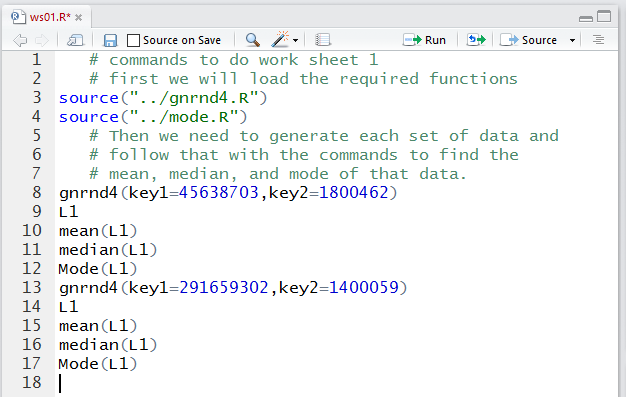
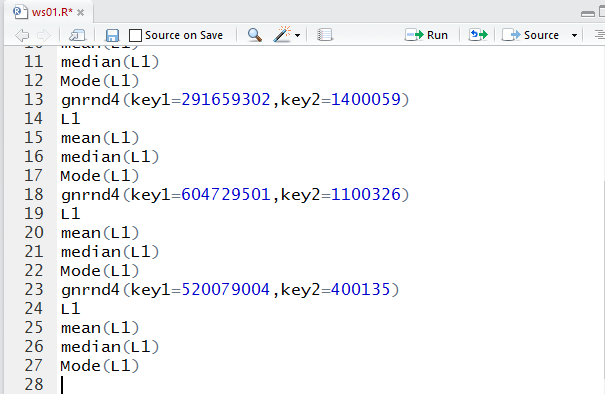
Figure 11 shows the Editor pane after all the lines have been entered.
Figure 11
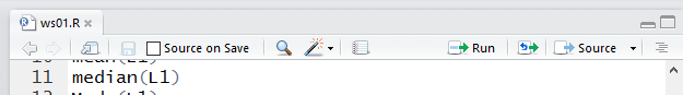
We notice that the name of the file, ws01.R
shown in the file tab is displayed in
red. That is an indication that the contents
of the file have yet to be saved.
We click on the  icon to save the file.
That will change the file name to be black, as we see in Figure 12.
icon to save the file.
That will change the file name to be black, as we see in Figure 12.
Figure 12
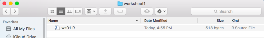
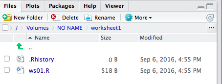
If we turn our attention to the lower right pane in the RStudio
window, and if we click on the Files tab there,
we will see that our file is there and that it holds the
518 bytes that we put into it.
This is shown in Figure 13.
You should notice that a second file also shows up.
That is the .Rhistory file that R
creates. It is a "hidden" file. We will not see it in
the Finder view of the folder.
Figure 13
Now we are ready to run all of the commands that we prepared.
We could highlight and run all of the commands in the
Editor pane, but if we did so we would have to scroll through the Console
display to see all of the results. Instead, here,
we will select just the commands that we want to see at each
step of the process.
Figure 14 shows that we can highlight the commands that load our functions (lines
3 and 4) and the commands to generate, view, and find the answers for
the data in table 1.
Figure 14
Once that is highlighted, we click on the
 icon to have those commands performed.
We can see the result in the Console pane, shown in Figure 15.
icon to have those commands performed.
We can see the result in the Console pane, shown in Figure 15.
We should verify that the values shown for L1 in Figure 15
are identical to the values we were given in 1.
Figure 15
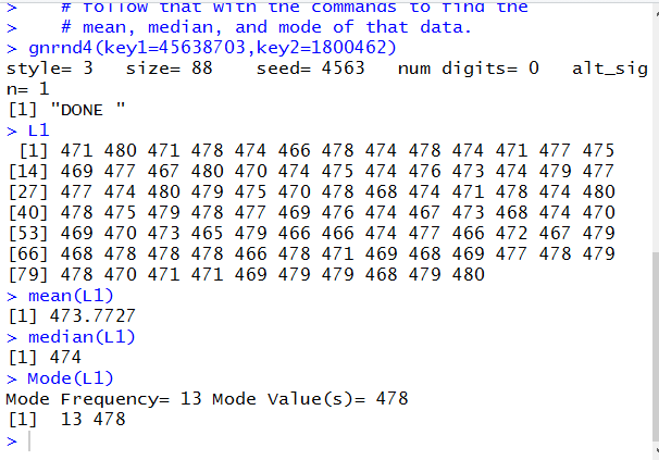
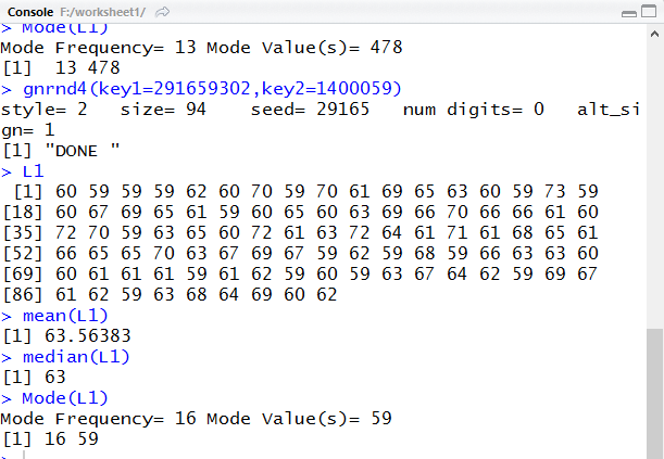
Then, reading the rest of Figure 15, w see that the
mean is 473.7727, the median is 474,
and the mode is 478, a value that appears 13 times
in the data.
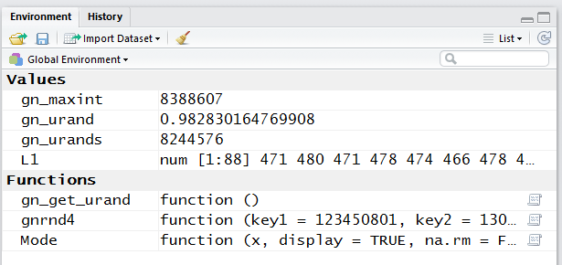
We should also note in the Environment pane, Figure 16,
that we have the variables and the functions that we expect to be defined.
Figure 16
Now we are ready to work with the data in Table 2.
Therefore, we highlight the appropirate commands in the
Editor pane (lines 13 through 17), as shown in
Figure 17. Then press the
icon.
Figure 17
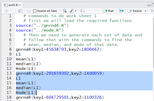
Figure 18 shows the results of thos commands.
Again we verify that the values displayed are identical to those in Table 2.
And we find that the
mean is 63.56383, the median is 63,
and the mode is 59, a value that appears 16 times
in the data.
Figure 18
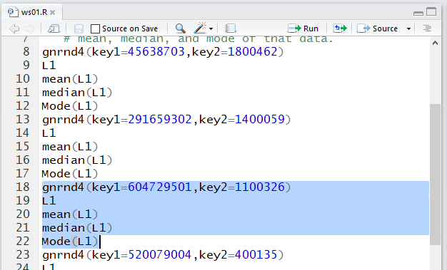
Returning to the Editor pane we highlight
the next set of commands.
Figure 19
Then we run them to get Figure 20.
Figure 20
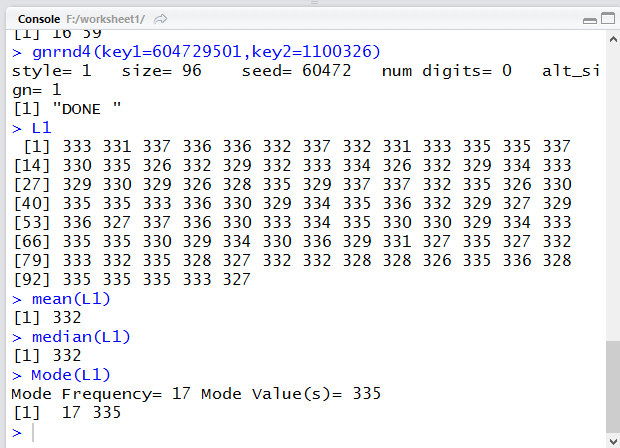
Again we verify that the values displayed are identical to those in Table 3.
And we find that the
mean is 332, the median is 332,
and the mode is 335, a value that appears 17 times
in the data.
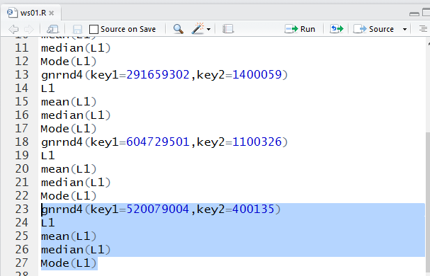
That leaves just the last set of commands to highlight, as shown in
Figure 21.
Figure 21
Then we run them to get Figure 22.
Figure 22
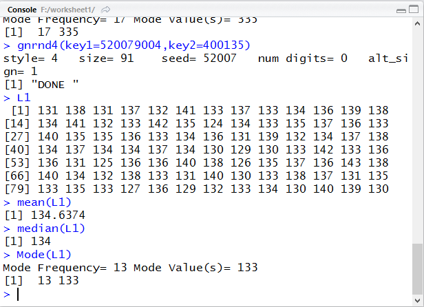
Again we verify that the values displayed are identical to those in Table 4.
And we find that the
mean is 134.6374, the median is 134,
and the mode is 133, a value that appears 13 times
in the data.
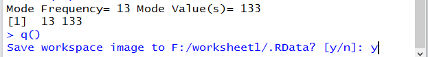
We have found all the values we needed to find.
Therefore, we can quit R via the q() command
shown in Figure 23.
Figure 23
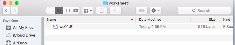
Once we have left RStudio, we can see, in
Figure 24, the Finder shows
that we have just one file in our directory.
Again, that is because the Mac hides files
with names that start with a period.
Figure 24
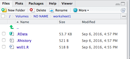
If we werre to restart RStudio, by double clcking on the
ws01.R file in Figure 24, then we woud see, in the Files
tab, all three files, as is shown in Figure 24.5
Figure 24.5
All that is left to do is to safely remove the USB drive.
We close the Finder window that is looking at our directory.
Then, pointing to the drive icon, ,
we can right click to open the menu shown in Figure 25.
Figure 25
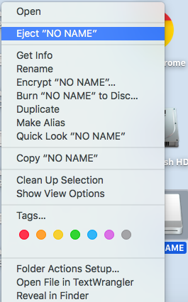
There we click on the Eject "NO NAME" option.
Once that is done, eventually, the USB drive icon on the desktop will
disappear. At that point we can safely remove the USB drive.
Return to Topics page
©Roger M. Palay
Saline, MI 48176 September, 2016