1. Insert the USB
2. Open the USB
3. Create a new folder (directory) on the USB
4. Give that folder the name "secondtry"
5. Copy the file "model.R" to "secondtry"
6. Rename this new copy of the file to "demo_two.R"
7. Start RStudio by double-clicking on "demo_two.R"
8. Verify the working directory via the getwd() command in the Console pane
9. Add new commands to the Editor pane
10. Execute those commands and observe the results
11. Move to the Files tab, observe entry
12. Save the Editor file
13. Observe the Files entry
14. Quit RStudio
15. Observe the contents of the "secondtry" folder
16. Start RStudio by double-clicking on "demo_two.R"
17. Observe the contents of the various panes in that window
18. Edit the "demo_two.R" file
19. Run the changed and affected commands
20. Observe the results
21. Save the file
22. Observe the Files tab contents
23. Quit RStudio

#  bring the gnrnd4 function into the workspace
#  from the parent directory
source("../gnrnd4.R")
#  generate the data
gnrnd4(key1=264899704, key2=700053)
#   just so that we can see all of the data we
#   use the command that is just the variable name
#   that holds the data
L1
#  get some computed values
summary(L1)
#  generate a histogram of the data
hist(L1)
#  bring the Mode function into the workspace
source("../mode.R")
#  find the mode of the data
Mode(L1)

The screen images on this page have been shrunk so that the web page is not extraordinarily long when viewing or printing it. Please note that on a Mac if you point to any of these images and right click on the image (or use the Control button and click on the image), then you have the option to view the image in its full size.

Insert the USB

Inserting the USB drive in my Mac computer eventually resulted in the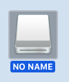 image appearing on the diesktop.

Open the USB

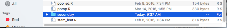
We double click on that image to open the drive. The result is the Finder window shown in Figure 1.

Figure 1

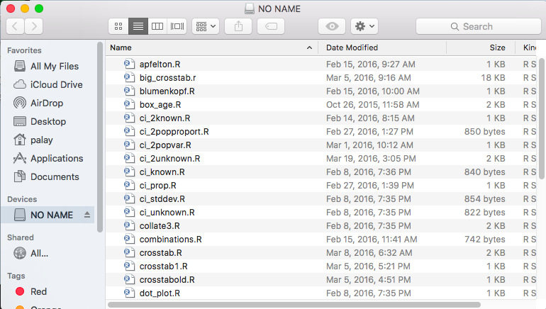
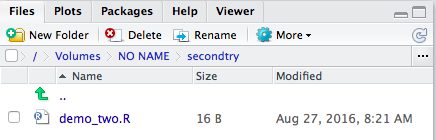
In the particular arrangement that we see in Figure 1, the existing folder (directory), firsttry, we see the start of the listing of the files that I distributed on the USB drive originally.

Create a new folder (directory) on the USB

Our next task is to create a new folder here. To do this we click on the File menu item in the Finder menu at the top of the screen. This causes the drop-down window shown in Figure 2 to open.

Figure 2

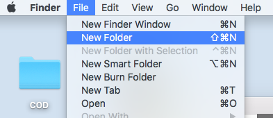
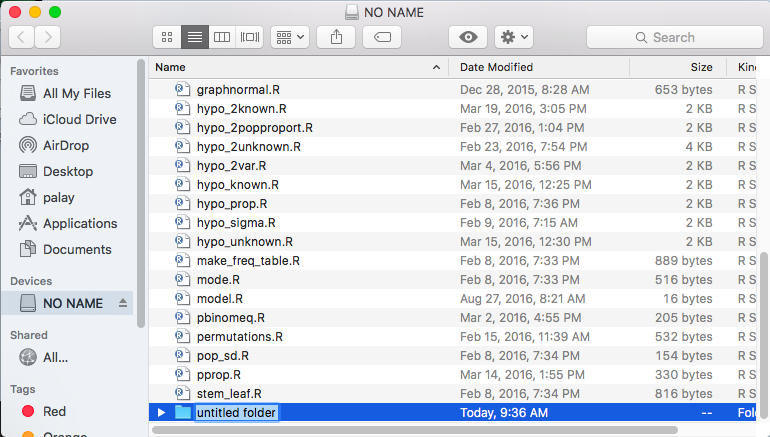
We click on the New Folder option in that drop-down window. This creates the new foder, shown in Figure 3, with the default name untitled folder.

Figure 3

Give that folder the name "secondtry

We can type in a new name for that folder. In Figure 4 we have entered the name secondtry.

Figure 4

Copy the file "model.R" to "secondtry"

Our next task is to make a copy of the file model.R and place it inot the newly created folder. If need be we scroll in the file list to find it. Once it is visibe, as in Figure 5, we point to it and right click on the name. That opens a small window of possibe actions, also shown in Figure 5. There we click on the Copy "model.R" option.

Figure 5

Having done that we have a copy of the model.R file. Now we need to navigate to the secondtry folder so that we can paste the copy there. To do that we locate the seondtry folder in the the Finder window. Then double click on that icon.

Figure 6

This will open the secondtry folder, as seen in Figure 7. It is of course, at this point, empty since we just created it. Point to the open area and right click there.

Figure 7

That should open the small window of possible operations shown in Figure 8. In that window, click on the Paste option.

Figure 8

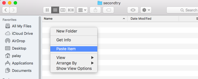
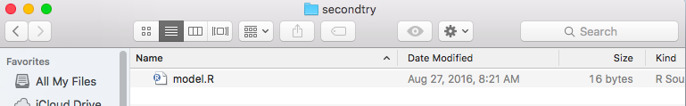
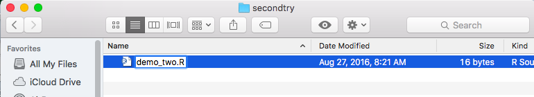
That will paste the copy of the file into this diretory as shown in Figure 9.

Figure 9

Rename this new copy of the file to "demo_two.R"

There are a numer of ways to start the process of changing the name of the file. One such way is to point to the file name, click on it, wait a second, click again on it. That is the action that caused Figure 9 to change to Figure 10.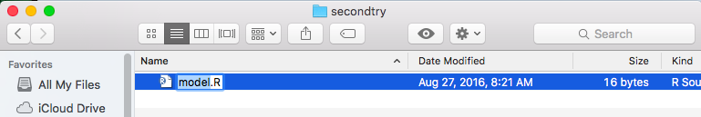

Figure 10

Once the name of the file appears in a small box, we can just type the new name of the file, as is shown in Figure 11. Once the name is typed we just press the Enter key.

Figure 11

With the name changed, the file appears as .

Start RStudio by double-clicking on "demo_two.R"

We double click on the file name to start a RStudio session with this as the working directory and with the demo_two.R file open in the Editor pane.

Unfortuanately, when I did this RStudio complained in the pop-up window shown in Figure 12, because a file I had been using the last time I used RStudio is no longer available. You may not get this error message and if you do not then just skip to the discussionb before Figure 13.

Figure 12

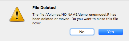
We really do not care about that problem, so we just repsond by clciking on the Yes button.

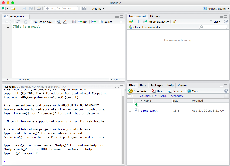
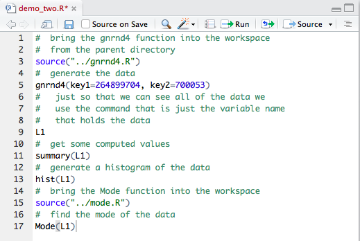
RStudio has been opened. Figure 13 shows the Editor pane in that session. The demo_two.R tab is open and the conents of that file are displayed, namely the one comment line.

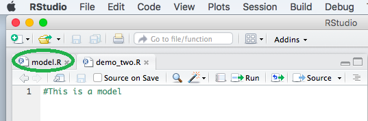
Again, unfortunately, I have another small mess to clean up. It would appear that the last time I used RStudio I left open a file called model.R, which I see in Figure 13 has its own tab, highlightd in an green oval. If you do not have a similar mess then you might want to skip down to the disussion just above Figure 15.



Figure 13

We can see what is in the model.R editor pane by clicking on that tab. When I did that on my machine I got Figure 14. I recognize this as the commands from the first demonstration. I do not need this at all. Therefore, I clicked on the small 'x' on the model.R tab. At that point the Editor pane should like like the image shown in Figure 14.

Figure 14

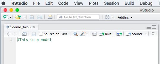
The full RStudio screen one shown in Figure 15.

Figure 15

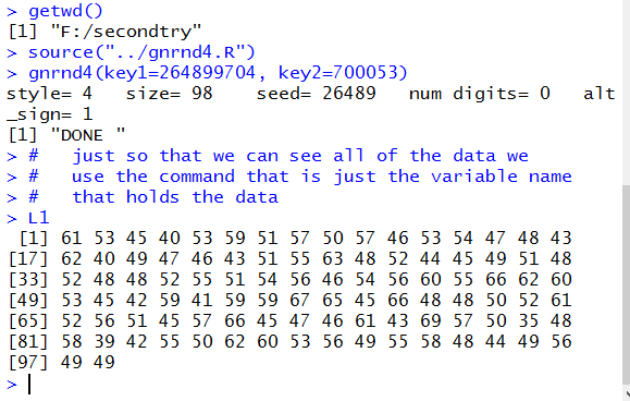
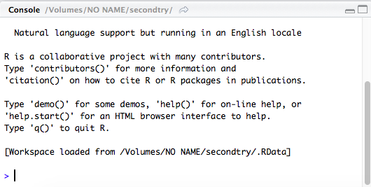
Verify the working directory via the getwd() command in the Console pane

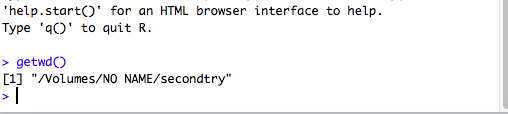
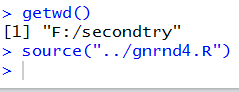
Just to be sure that everything is as I want it to be, I use the getwd() command in the Console pane. Once I type the command and press the Enter key, R lets me now that the current working directory is /Volues/No Name/secondtry. This shown in Figure 16.

Figure 16

Add new commands to the Editor pane

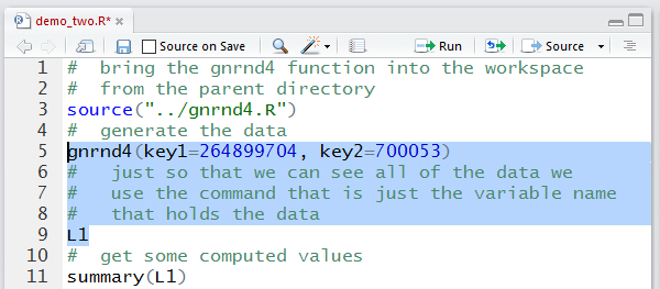
We want to take the commands given much earlier on this page and place them into the editor. We could, of course, just tyoe them into the Editor pane. However, that is a good deal of typing and it is an invitation to introducing errors. Rather, we can go back on this page to find the ommand and highlight then as shown in Figure 16.3 below.

Figure 16.3

Once they are highlighted we can copy them (Ctrl-C). Then we return to the RStudio window, and in the editor we highlight the existing comment and then replace it by the new commands by pasting (Crtl-V) them there. This produces Figure 16.6 below.

Figure 16.6

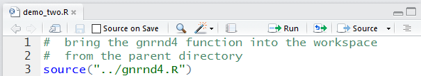
Execute those commands and observe the results

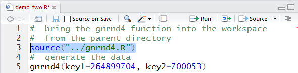
Now we can start to perform the commands. To perform the source("../gnrnd4.R") we just need to highlight it as shown in Figure 17.

Figure 17

Then we click on the icon to execute that command. This will paste the command into the Console pane and then run it. The result shown in the Console pane is given in Figure 18. There is not much there other than not having an error message.

The command source("../gnrnd4.R") tells R to look in the parent folder (that is what the ../ means) for the file gnrnd4.R and to run the commands found in that file. That file, should you want to look at it, is over 400 lines long. However, it boils down to defining two funtions and two variables. Because it is only definitions, it does not produce any output.

Figure 18

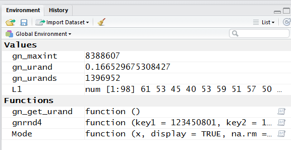
In Figure 19 we can see that we do have two variables defined and two fnctions defined where one of the functions happens to be called gnrnd4. (There is no need to have the name of the file and the name of the function be the same, but it does help to identify what is in a file to have that be the case.)

Figure 19

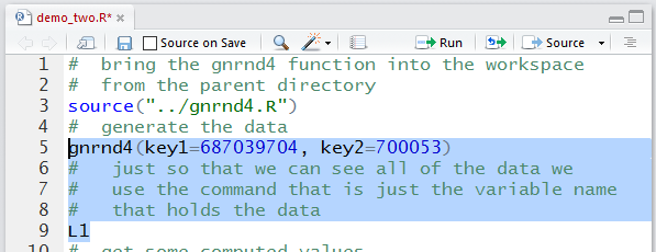
We return to the Editor pane and highlight the next two commands, along with the comments between them. The first command, gnrnd4(key1=264899704, key2=700053) runs the function, gnrnd4, that we just defined. That function generates lists of values as determined by the key vaues that we give it. [I have a similar function in my web pages, written in Javascript not R, so that I can produce values in the web pages and have students be able to produce the same values within ther R session. This saves students from having to enter longs lists of values.]

The second command, L1, is just the name of a variable. When R is just given the name of the variable R tries to display the values stored in that variable.

Once we have highlighted the lines, we click on the icon to execute those commands.

Figure 20

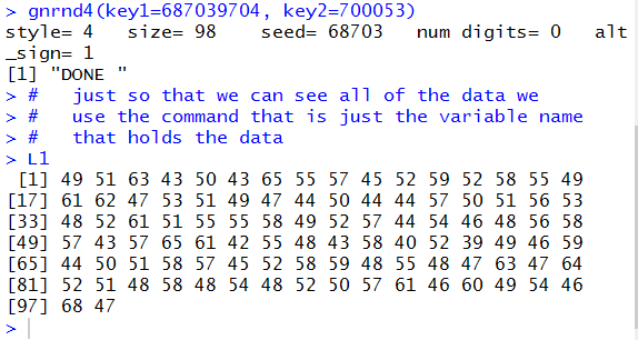
We can see the result in the Console pane shown in Figure 21. We can compare the values displayed for L1 in Figure 21 with the values that were in the table given at the start of ths web page and we see tht with the one call to the gnrnd4 function we were able to generate all 98 values.

Figure 21

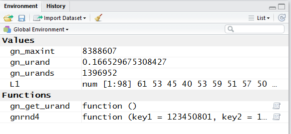
We we look at the Environment pane we see that L1 is now defined and we see that it holds numeric values, and that there are 98 such values. In addition, we can see the first few of those values.

Figure 22

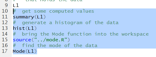
Then we can highlight the rest of the commands back in the Editor pane. Of those, the command summary(L1) causes R to find and display six important values related to the 98 values in L1. The six values are the minimum value, the first quartile value, the median value, the mean value, the third quartile value, and the maximum value. [Soon, in this course we will talk about each of these, how they are computed, and how we use them. At the moment, we are just happy that R finds them with such ease.

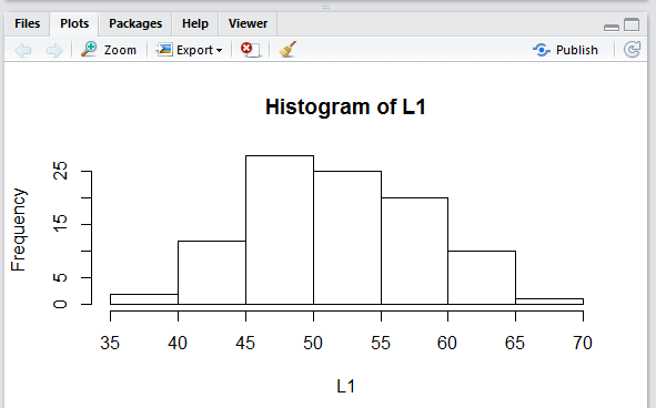
The next comman is hist(L1). That command causes R to produce a histogram of the values in L1. This graph appears in the RStudio pane Plots.

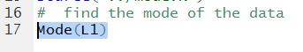
Following that we want to find the mode of the values in L1. R does not have a command to do this, but I wrote a function definition that we can use. You have that definition on the USB drive, in the file called Mode.R, which is in the parent directory. Therefore, we use the command source("../mode.R") to load that function definition into our workspace. After we have done that we can use the command Mode(L1) to have R find the mode value(s) for the data stored in L1.

As usual, once the commands are highlighted, we click on the icon to execute those commands.

Figure 23

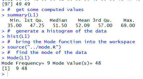
In Figure 24 we see the six summary values. The hist(L1) command does not produce anything in the Console pane, but as we will see in Figure 26, it does produce a nice looking histogram. The source("../mode.R") also does not produce any output in th Console pane, though we will see, in Figure 25, that a new function has been defined. The Mode(L1)command produces some output. In this case that output tells us that the value 48 is in L1 9 times and that n other vaue appear that often or more often.

Figure 24

In Figure 25 we see the small change in the Environment pane, namely, the addition of the Mode funtion.

Figure 25

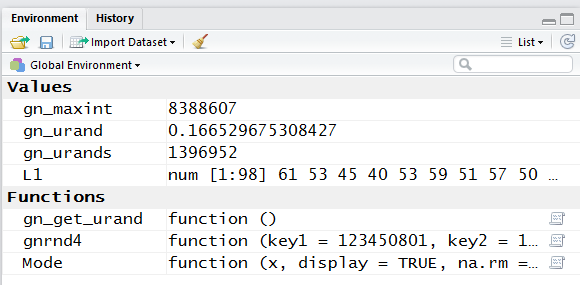
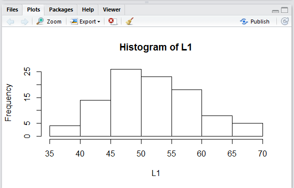
Figure 26 shows the Plots tab in the lower right pane of our RStudio window. There we see the histogram that we asked R to produce.

Figure 26

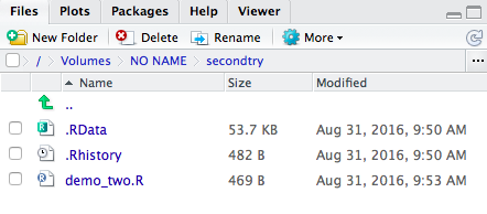
Move to the Files tab, observe entry

This would be a good time to pause for a moment and examine the files in our workspace. To do this we open the Files tab in the lower right pane of the RStudio window. There we see the demo_two.R file, just as we had it once we renamed it. All of our work in the Editor pane has stayed there. It has not yet been saved.

Figure 27

Save the Editor file

To actuall save our work, that is save the text in the Editor, we return to that pane. There, as shown in Figure 28, we actually see the red name of the file indicating that changes have been made but the file has not been saved.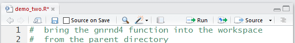

Figure 28

To now save the file we click on the icon. The only difference that we see in the Editor pane is that the color of the name of the file has changed from red to black.

Figure 29

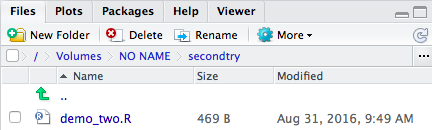
Observe the Files entry

However, if we look in the Files tab, shown in Figure 30, we can see that the file has changed. It is now larger and it has a new timestamp.

Figure 30

Quit RStudio

That is enough for the moment. We move to the Console pane and type q(), press the Enter key, and then respond with y to get Figure 31.

Figure 31

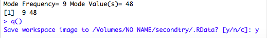
Once we then press the Enter key, RStudio will close down after saving the workspace.

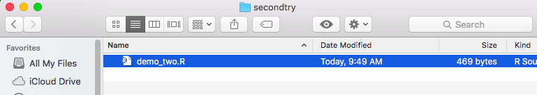
Observe the contents of the "secondtry" folder

We should then be looking at the Finder window showing our secondtry folder. That is shown in Figure 32. On a PC we would see three files now, but on the ac we only see one. The demo_two.R file is there as expected. The two non-visible files are .RData and .Rhistory. The .RData file holds the workspace values. In particular, it holds all the variables and all the function definitions. The .Rhistory file holds a list of the commands that we asked R to perform. These are "hidden" files and on a Mac, by efaut, hidden files are not shown in the Finder listing. We, however, will be able to see them in RStudio when we restart that program.

Figure 32

Start RStudio by double-clicking on "demo_two.R

To see why it is helpful to have the saved workspace, we just need to retart RStudio from this same directory. We can do this, from Figure 32, by double clickng on the name of the demo_two.R file.

Observe the contents of the various panes in that window

This will start a new RStudio session. In that new session, we find, in the Editor pane, shown in Figure 33, our file already for any further modification.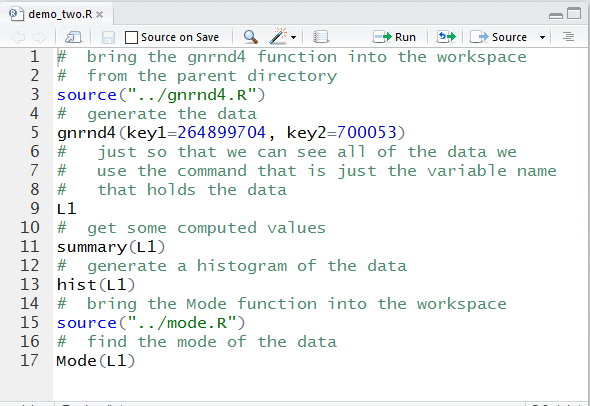

Figure 33

In the Environment page, shown in Figure 34, we see all of our old variables, with their same values, and our function definitions.

Figure 34

In the Console pane, Figure 35, we just find the start of a new R session, although it does tell us now that the workspace has been loaded from our .RData file.

Figure 35

The Files tab shows the files in our working diretory, including the "hidden' files that did not show up in the Finder window back in Figure 32. This is shown in Figure 36.

Figure 36

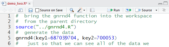
We will make a small change now. It turns out that, somehow, I made a small mistake when I first started this page. The table at the top of the page was the wrong table. It should have been



We note that the only change we need to make is in the values for the first keyfor our gnrn4 function call.

Edit the "demo_two.R" file

We can make that change by looking at the Editor pane,. This is shoen in Figure 37 where we have hghlighted the old, wrong value, in that command.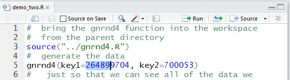

Figure 37

We enter the new value, the 68703, as the first part of the first key value to get to Figure 38.

Figure 38

Run the changed and affected commands

Because the functions have already been loaded as part of the worspace, we do not need to load them again. Therefore, in Figure 39, we just highight the two statements that generate the valus and then display the values. once the commands are highlighted, we click on the icon to execute those commands.

Figure 39

Observe the results

In Figure 40 we see that indeed the gnrnd4 function ran and it produced the desired new values, the ones that match our new table values.

Figure 40

We get new summary values and a new histogram by highlighting thse command and then clicking on the icon to execute those commands.

Figure 41

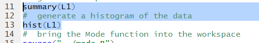
Figure 42 shows the new results. which are, of course, different from the results we got with the earlier table of values.

Figure 42

Figure 43 has the new histogram in the Plots tab. It, to, is different from the old histogram, back in Figure 26.

Figure 43

Again, because the Mode function is already defined in our workspace we do not need to load it again. Instead we can just highlight the command and press icon to execute it.

Figure 44

This is a very differenet result. now there are two mode values, 48 and 52, both of which occur 8 times in the new table of values. We see this in the output shown in Figure 45.

Figure 45

Save the file

We return our attention to the Editorpane, Figure 46. There we note that the file has been changes, so the file name now appears in red.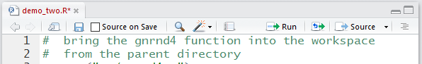

Figure 46

Click on the icon to save the file. That changes the color of the file name to indicate that this is the current value of the saved file. We see this in Figure 47.

Figure 47

Observe the Files tab contents

When we look at the Files tab we see that the timestamp has changed.

Figure 48

Quit RStudio

We are done for now so we type the q() command into the Console, press the Enter key, and respond with a y to indicate that the workspac should be saved. That is shown in Figure 49.

Figure 49

We conclude by pressing the Enter key. R saves the workspace and RStudio closes.

Return to Topics page
©Roger M. Palay     Saline, MI 48176     August, 2016