Using gnrnd4 on a PC
Return to Topics page
This page describes the purpose of and the use of a set of routines encompassed
in the file gnrnd4.R. The purpose and use are strictly related
to the material of this course and, in particular, to the coordination of
data values on many of the web pages in this course and
obtaining the same values in an R session.
There are many times when web pages in this course
make reference to a collection of data values.
For example, consider the
Now, although the particular web page may wish to talk about
this data, it would be even better, and in the case of tests on web pages it may be
highly desirable, if you could create a vector of the same values on
your computer, and to do so in R.
If the web page is being displayed on a computer, then one
possible solution would be to highlight the data in the table,
copy it, and paste it to a file.
Were we to do that then the file would have
values in a number of rows and in a number of columns.
R would have a hard time reading that directly, but we could manage it, with
a lot of extra work.
We would have to find some way to read that into R.
Another solution would be to copy the contents of the table
and paste it into some program such as Microsoft Excel,
where we could manipulate the data until we could write it
to a file in a form that R could read.
Of course, neither of those solutions would be of any help
if we were reading Table 1 on paper, as might be the case for a test.
The obvious solution would be to just type the values into R.
The command to do this is:
But who wants to type that?
In fact, I am sure that I couldn't type that without making at least one error!
One interesting note here is that rather than being presented in table format
if the values were presented as a
comma separated list, such as we just saw in the command above, then we
would have an easier time, using Excel, in converting them to a form
that we could eventually read into R.
But that still does not help in the printed version of the collection of values.
The values given in Table 1 above are generated each time the page is loaded or refreshed
by a Javascript program that is part of this web page.
In fact, if you were to use your browser to look at the page source
then you would be able to find and read that Javascript program.
Since the numbers in our table were generated by a program, it would be
really nice if we had a R script that would generate the same values
for us in R.
The gnrnd4() function, written in R,
performs exactly the same computations as did the Javascript program.
The gnrnd4() function is provided in the
file gnrnd4.R. The trick is
- to get that file
- to load it into R
so that you can use it
- to give the R function the starting point
used by the Javascript program to generate the values.
There are a number of ways to achieve points 1 and 2.
On my web page there is a listing that gives all of the
routines that I have written for this course.
It is on the page
Table of Links to various R scripts.
Part of that table provides a link to each of the routines.
You could use that link to download the file to your computer
and then
copy it into any R session that you are using.
A second approach would be to use a R
command that would directly read the file from my web site.
The R command to do that is
source("http://courses.wccnet.edu/~palay/math160r/gnrnd4.R")
The third approach, and the one I want us to use,
just imports the function from the file that we
installed onto your computer in our first class meeting.
You can have R load the file from that drive.
The steps that follow walk you through doing this.
The numbers in Table 1 change each time you load or refresh this page.
In order to demonstrate here with images of our RStudio work
we need to have a static set of values. So here is a new set of values.
Our goal will be to generate the values in the following table:
The eventual command that we will use to generate these same values
in our R session is
gnrnd4(key1=364527804,key2=1600123). However, we
want to do a number of steps first.
The work here was done on a PC running Windows 10.
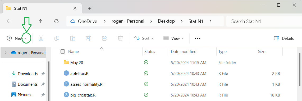
We start by clicking on our desktop folder for this class.
This opens
File Explorer (or Finder on a Mac) to give us a view of the contents of that folder.
The top of that view is shown in Figure 0. I have put a green
circle around the down arrow after the word New in that image.
Figure 0
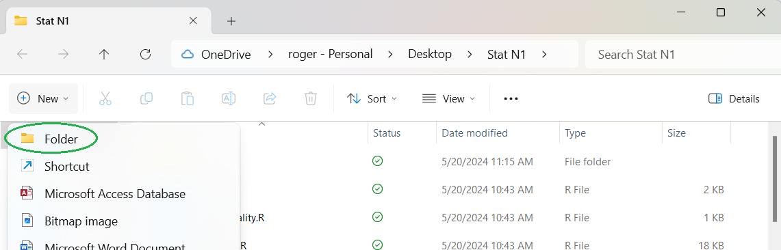
Within that menu we want to click on the down arrow circled in Figure 0.
That opens the list of options shown in Figure 1. Again I have added green oval
around the next step, Folder.
Figure 1
This creates a new folder with the default name New folder,
a name we would like to change now.
Figure 2
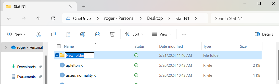
Because the name New folder is highlighted in Figure 2
we can just enter our new name; in this example we will
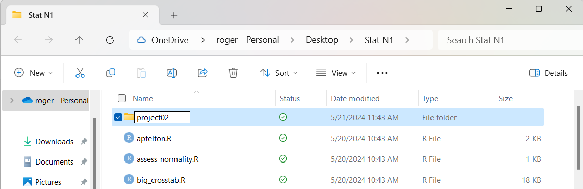
call it project02, as shown in Figure 3.
Figure 3
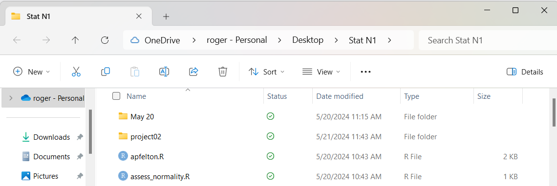
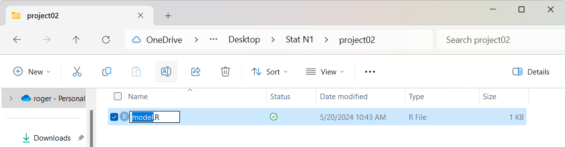
Our next step is to get a copy of the file
model.R from the folder.
Figure 3 is still displaying that folder.
Therefore, we scroll to display the file name, model.R,
and point to and click, just one time, on that file name. This highlights
the line containing the model.R file as shown in Figure 4.
Again, I have added a green circle to show our next step.
Figure 4
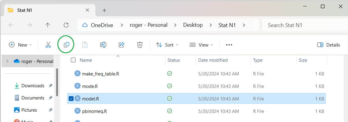
Now to make a copy of that model.R file
we just click on the option in the green circle of Figure 04.
At this point the computer has a copy of the file.
We want to put that copy into our new folder, project02.
To do this we need to navigate to that new folder.
We do this by first scrolling to find the folder
as shown in Figure 5.
Figure 5
Then we just double-click on the name of the folder,
in this case, project02.
This causes File Explorer to display the contents
of the project02 folder, shown in Figure 6.
As before, I have added a green circle to show our next step.
Figure 6
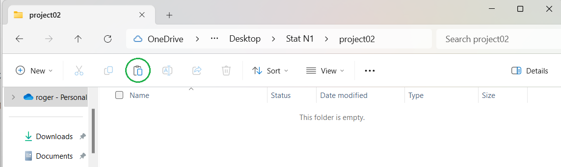
As expected, since we just created the folder, it is empty.
But not for long.
Now click on the option circled in green in Figure 06
to paste the file into our new folder.
This is shown in Figure 08
Figure 8
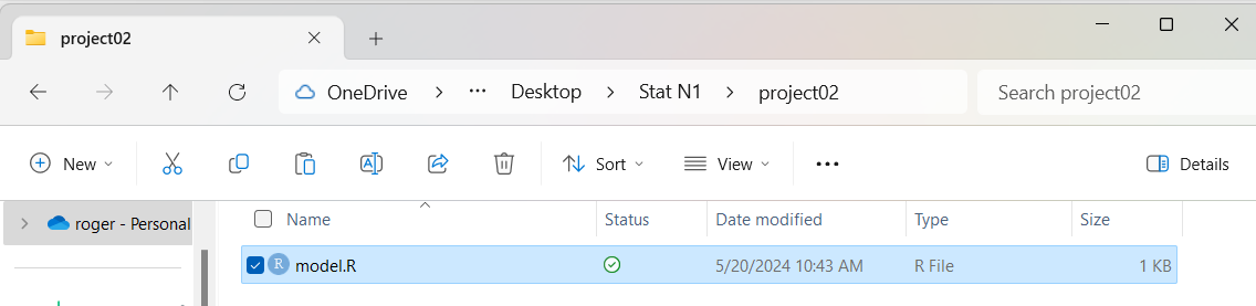
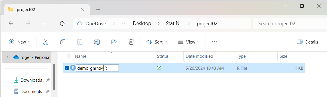
Now we want to rename the file to
something more appropriate. We point to the model.R
file in Figure 8, click one time on it, and then click on
the option in the green circle in Figure 08.
This will highlight just the base part of the file name, as shown in Figure 09.
Figure 9
Then type in the new name,
we will use the name demo_gnrnd4.R
and we get Figure 10.
Figure 10
Then we double click on that file name
in order to open our RStudio session.
Figure 11 shows the entire RStudio window.
Figure 11
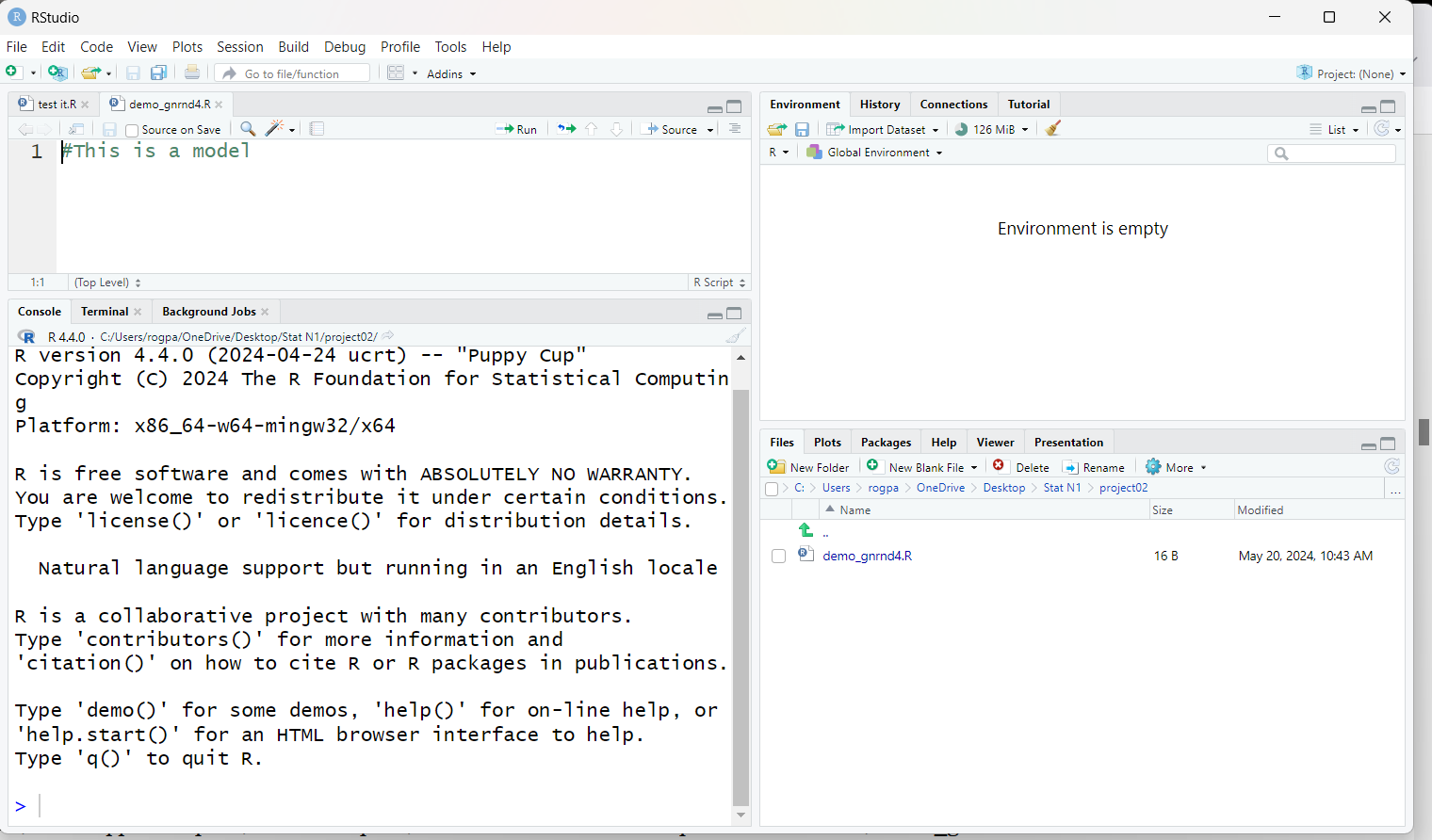
If we look, in Figure 12, at the upper left pane, the editor pane,
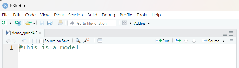
we see that RStudio has opened our new file, demo_gnrnd4.R.
Figure 12
Note, in Figure 12, that there is another file,
in this instance test it, that is in the editor.
This is left over from an
earlier run of RStudio. We do not want this file in this session.
Therefore, we click on the little "x" after that file
name in order to close it. That leaves us with just the
demo_gnrnd4.R file in the editor, as shown in Figure 13.
Figure 13
If we turn our attention to the
lower left pane of Figure 11, we see Figure 14.
Figure 14
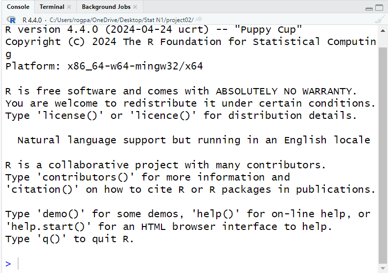
Figure 14 shows the console dispaly for the version of R
that is running on our computer. This is where we will see the results of all of the
R commands that we will give.
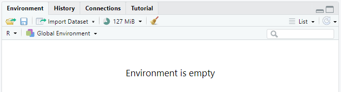
At the top right of Figure 11 we find
the environment pane, shown in Figure 15.
Because we have created a new folder and because we have started RStudio
from that new folder, the environment starts out empty.
We are starting with a clean slate.
Figure 15
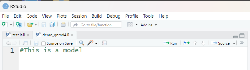
Returning to the editor pane, we want to type some new comment lines
and then type the one command source("../gnrnd4.R") as shown in
Figure 16. To make life a bit easier for you, the lines are
#This is an example of using gnrnd4.
#   I have a web page that tells me that I can generate
#   specific data values in a given table by using
#   the gnrnd4 routine with given arguments.
#   I will try it here.

#  First we need to get the gnrnd4 routine into our
#  current environment.  the routine is on this USB
#  drive, in the directory (folder) directly above
#  this one.  So we use the command

source("../gnrnd4.R")
If you are following along on your own computer you can copy
the lines from this web page and just paste them into your
RStudio session.
Figure 16
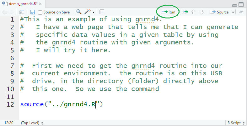
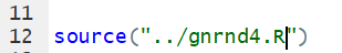
Figure 17 shows just lines 11 and 12 of Figure 16.
Notice that the cursor is on line 12,
the line containing the command that we want to run.
To run that command click on the
 at the top of the
editor pane, circled back in Figure 16.
at the top of the
editor pane, circled back in Figure 16.
Figure 17
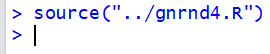
The result, shown in the console pane in Figure 17a,
is that the command is run in R. It produces no output.
Figure 17a
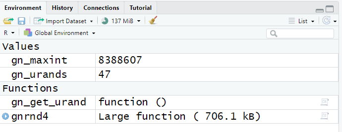
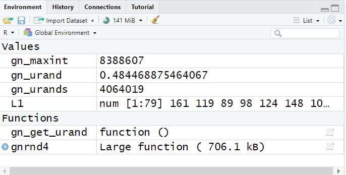
However, if we return to the environment pane,
Figure 18, we see that two new values and two new functions
have been defined.
Figure 18
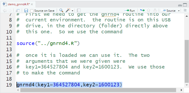
Now that the function has been loaded into our environment we can
actually use it. Figure 19 shows the new lines that we have
added in the editor pane. They are reproduced here so that you can copy them if so desired into your
RStudio session.
#  once it is loaded we can use it.  The two
#  arguments that we were given were
#  key1=364527804 and key2=1600123.  We use those
# to make the command

gnrnd4(key1=364527804,key2=1600123)
Figure 19
In Figure 19 we have hghlighted the command that we actually want to execute.
We click on the to actually run that hghlighted command.
The result is seen, in the console pane, in Figure 20.
Figure 20
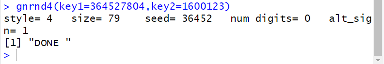
This time there was actually some output, but its meaning is not
completely clear. On the other hand, if we look back at the
environment pane, shown in Figure 21, we see that we now have two new
variables, one of which, L1, seems to hold the
numbers from Table 2 that we were trying to
create in our RStudio session.
Figure 21
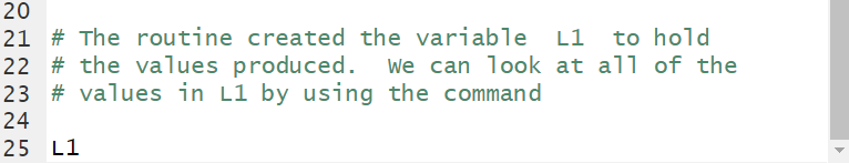
If we want to see all of the contents of L1 we can just use
that variable name. As has been our practice we will first add it to the editor
pane. That is done in Figure 22.
Figure 22
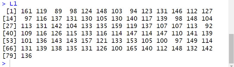
Then, using the ![]() we have
RStudio perform that command in the console
pane shown in Figure 23.
we have
RStudio perform that command in the console
pane shown in Figure 23.
Figure 23
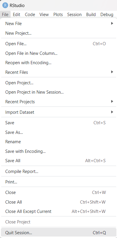
At this point we are essentially done. We can
quit by clicking on the File menu option and then
clicking on the Quit Session option as shown
in Figure 24.
Figure 24
When we try to quit the session RStudio recognizes that we have been adding things to
the file in the editor, namely, to the file demo_gnrnd4.R.
RStudio does not want us to accidently lose our work so it gives
us the option, shown in Figure 25, to save that file.
Figure 25
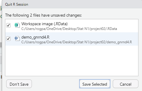
Once we click on the Save Selected button in Figure 25 RStudio
ends.
This returns us to the File explorer
screen which now shows the current
contents of our folder project02.
Figure 27
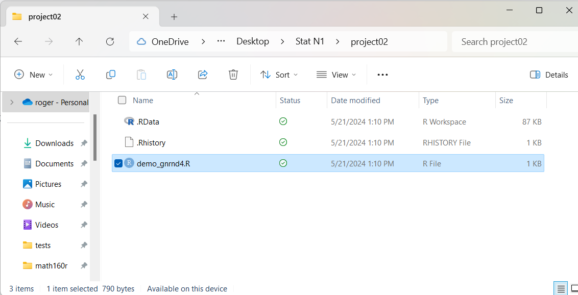
The contents of Figure 27 may seem a little strange. First of all, for PC users,
there are now three
files in the folder. The file demo_gnrnd4.R is expected. You might note that it has now
grown to be 1KB long. The other two files remain a bit of a mystery.
The .Rhistory file contains the list of commands that were given in our session.
The .RData file contains the environment.
Note that Mac users will not see in Finder the hidden files but they are still there.
The beauty of this is that if we
double click on the demo_gnrnd4.R file,
we will start a new RStudio session, but this time it will start with the environment
the way we left it back in Figure 26. You can see this in Figure 30.
Figure 30
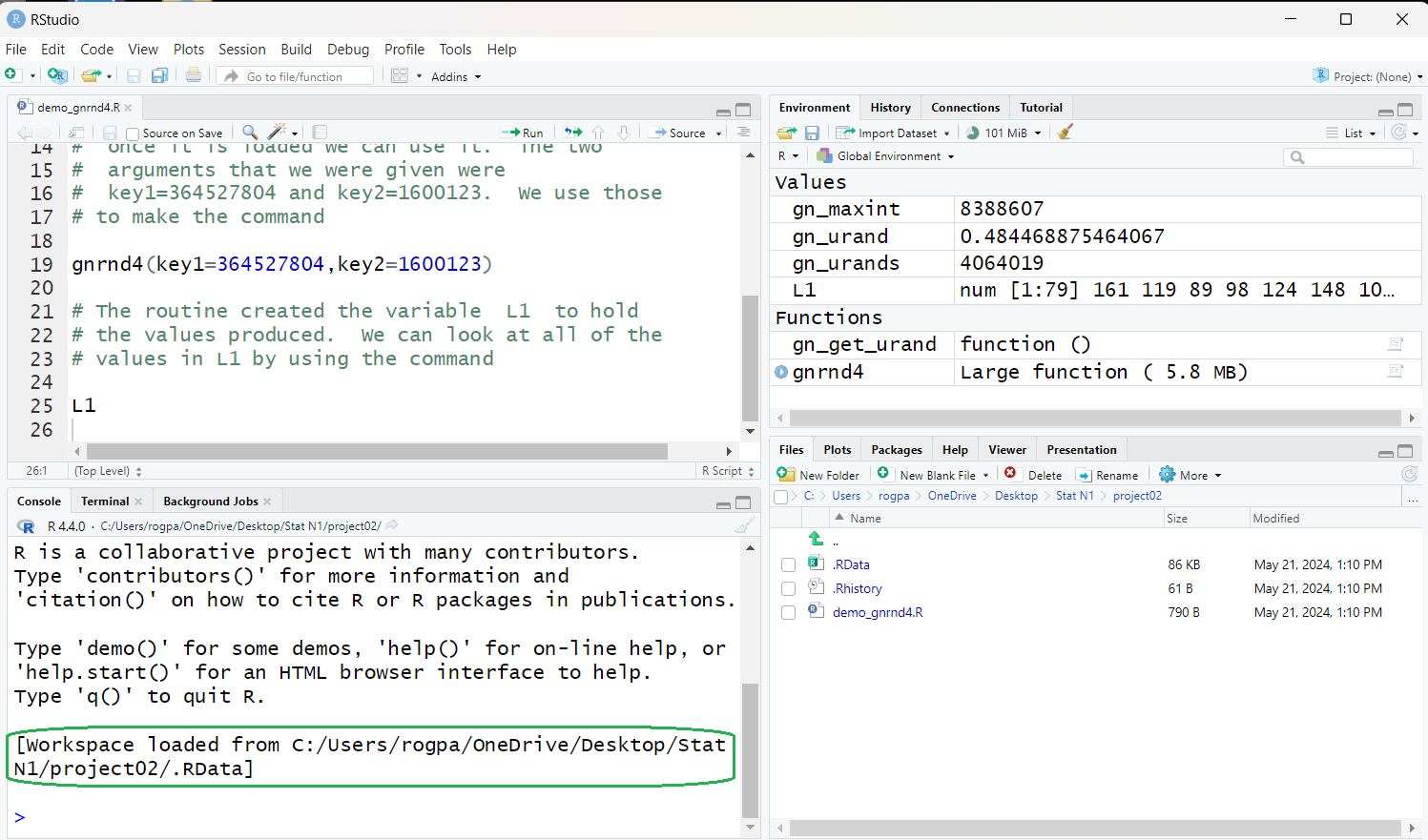
Pay particular attention to the notice in the green outlined area
where we see that the environment has been loaded from
the .RData file in our folder.
We close our RStudio session as usual.
Here is the list of commands used on this page:
#This is an example of using gnrnd4.
#   I have a web page that tells me that I can generate
#   specific data values in a given table by using
#   the gnrnd4 routine with given arguments.
#   I will try it here.

#  First we need to get the gnrnd4 routine into our
#  current environment.  the routine is on this USB
#  drive, in the directory (folder) directly above
#  this one.  So we use the command

source("../gnrnd4.R")

#  once it is loaded we can use it.  The two
#  arguments that we were given were
#  key1=364527804 and key2=1600123.  We use those
# to make the command

gnrnd4(key1=364527804,key2=1600123)

# The routine created the variable  L1  to hold
# the values produced.  We can look at all of the
# values in L1 by using the command

L1
Return to Topics page
©Roger M. Palay
Saline, MI 48176 May, 2024