Sampling -- Simple Random Sample

Return to the Sampling page

A Simple Random Sample, sometimes referred to as a SRS, is a sample drawn in such a way that every item in the population has an equal chance of being selected. This equal likelihood of being selected must remain essentially true even after some items in the population have been selected. Another way to look at this is that if we are in the middle of the selection process, then knowing that a particular item has already been selected tells us nothing about the likelihood that any other item will be selected next.

For example, in the fall term of 2013 let us say that there were 11,413 registered credit students at the community college. If we have a list of those students, one student per line, then we could use a random number table, or more likely, a random number generator on a computer, to select a sample of 60 students. We would just be selecting items from this long list of students. Each student has an equal chance of being selected for the first spot in our sample. After selecting that student, then the 11,412 remaining students have an equal chance of being selected for the second spot in the sample, and so on. Knowing that any one student has been selected does not help you make any better guess about whether or not some other student has been or will be selected.

We note that even though an approach may "look like" it is a simple random sample, the details of the process may force us to recognize that such is not the case. For example, it is quite easy to get the list of credit students at the community college by just getting the class lists for all credit classes. If we did this we might find that there 35,819 such entries. What if we selected our 60 student sample from that list of 35,819 items? If we are interested in getting a simple random sample of credit students at the college, then this methodology does not work. A student who is enrolled in four classes has four times the likelihood of being selected as does a student registered for just one class. Such an inequality of the likelihood of being selected indicates that this methodology does not give us a simple random sample.

On the other hand, if we are looking for a simple random sample of "registrations" then this methodology is exactly what we want to do. (We might note that as a researcher we would have to tackle the unlikely but real possibility that the same students might be selected for two different registrations. That may, or may not, be a concern to the researcher.) However, the previous plan, selecting 60 random students first, and then going from there to select a regisitration from those identified students is not going to be a SRS for getting a sample of registrations.

To see how we can do a SRS in R let us consider an example. Table 1 holds 98 values. We will look at a process to randomly select 10 of those values.
The following commands generate that same data in R and both display and summarize the data.

gnrnd4( key1=2765929704, key2=0342313872 )
L1
summary(L1)

The console output from those commands appears in Figure 1.

Figure 1

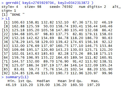
Figure 1 shows that we have generated the data, now stored in L1, and we can even use that data in a command such as summary(L1).

We can use the command sample( L1, 10, replace=FALSE) to take a sample of size 10 from the values in L1. The commands

samp_1 <- sample( L1, 10, replace=FALSE)
samp_1
samp_2 <- sample( L1, 10, replace=FALSE)
samp_2
samp_3 <- sample( L1, 10, replace=FALSE)
samp_3

will cause R to take three such samples and store them in samp_1, samp_2, and samp_3, respectively. The commands also cause the samples to be displayed. The result, which is almost certainly different from a result you would get if you were to run the commands on your machine, is given in Figure 2.

Figure 2

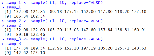
Indeed, the commands shown in Figure 2 are merely three successive calls to the function sample(), with each call being the identical code sample(L1,10,replace=FALSE). And, yet, the result of each one of the three calls is a different sample of size 10 the original 98 value. [And if you performed the same commands you would, almost certainly, get three other simple random samples.]

This is exactly what we want. Each time we use sample(L1,10,replace=FALSE) we want R to perform a SRS to get a new sample from the data. We should note that the values generated in Figure 2 represent 3 different simple random samples. That does not mean that the three samples do not overlap. In fact the values 89.18, 132.08, and 147.80 appear in both samp_1 and samp_2, the value 177.10 appears in samp_1 and samp_3, while the value 105.20 appears in both samp_2 and samp_3. It is possible for two SRS's to produce the same samples, but this is highly unlikely (unless we play around with the seed of R's random number generator. We will do that below under Setting the Seed.

What then is the meaning of replace=FALSE in the command sample(L1,10,replace=FALSE)? Samples can be taken with replacement or without replacement. If we take a sample without replacement, and this is the meaning of replace=FALSE, then once an item has been selected it cannot be selected again. It is removed from the list of potential values to be sampled. In our current example, where we start with 98 values, selecting the first value leaves 97 possible choices for the second. Selecting that second value leaves 96 choices for the third, and so on. Obviously, in this case, we could not take a sample of size 130 from our original data because we would have used up all possible values as soon as we found our 98^th value. There would be nothing left to select for the 99^th.

If we take samples with replacement then after an item is selected it is left in the collection of possible values. In fact, it could be selected again. We will look at sampling with replacement later.

As noted above, unlike other images that you have seen in these pages, at least up to this point, if you run the commands given above, that is

gnrnd4( key1=2765929704, key2=0342313872 )
L1
summary(L1)
samp_1 <- sample( L1, 10, replace=FALSE)
samp_1
samp_2 <- sample( L1, 10, replace=FALSE)
samp_2
samp_3 <- sample( L1, 10, replace=FALSE)
samp_3

You will find that R produces the same collection of values in L1 but, almost certainly not the same values in samp_1, samp_2, and samp_3. This randomness is controlled by a seed value that R maintains. That seed value changes every time R produces a random value. Given the commands that we have used so far we have no idea what the value of the seed is when we start asking for our three SRS's. As a result, we will get different SRS's each time we perform the same sample() commands.

Setting the Seed

That randomness is both good and bad. It is good, because we really want truly random samples. It is bad because it means that we cannot reproduce our results and others cannot exactly replicate what we have done.

To reach a middle point between the extremes of total randomness and total predictability, R allows us to set the seed value. We do this with the set.seed() function. For example, assuming that we still have the same values in L1, the sequence of commands

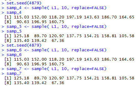
set.seed(4879)
samp_4 <- sample( L1, 10, replace=FALSE)
samp_4
samp_5 <- sample( L1, 10, replace=FALSE)
samp_5
set.seed(4879)
samp_6 <- sample( L1, 10, replace=FALSE)
samp_6
samp_7 <- sample( L1, 10, replace=FALSE)
samp_7

will

set the seed value to 4879
produce and display two simple random samples, samp_4 and samp_5 (during this process the seed value will be changing over and over)
reset the seed value to 4879
produce and display two simple random samples, samp_6 and samp_7 (again, during this process the seed value will be changing over and over)

However, because we initially set the seed and then reset the seed the SRS in samp_4 is identical to the SRS in samp_6 and the SRS in samp_5 is identical to the SRS in samp_7. We can see all of this play out in Figure 3.

Figure 3

Again, assuming that you have used the earlier gnrnd4() function call to produce the values of Table 1 in L1, if you issue the same commands as shown in Figure 3 on your computer then you will get exactly the same values in samp_4, samp_5, samp_6 and samp_7 as are shown in Figure 3.

Once you have used a set.seed() statement you have firmly determined the sequence of random values that R will generate from then on in the R session. If, by chance, you want to return to the unknown, non-reproducable, sequence of random values then issue the set.seed(seed=NULL) command and R will re-initialize its seed value as if you had never set the value yourself.

With Replacement

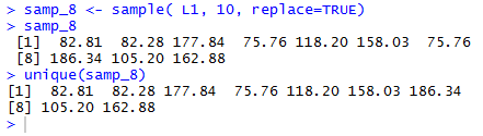
The alernative to the sampling without replacement shown above is sampling with replacement. To get R to sample with replacement we change the parameter when we call the function to replace=TRUE. In Figure 4 we can see the creation of values in samp_8 by using samp_8<-sample(L1,10,replace=TRUE) . At first glance the result does not seem different that the SRS's produced above. However, as luck would hve it, this particular call to sample() yieldedvalues where we have selected the same value, namely, 75.76, twice. That value did not appear twice in Table 1. Rather, the sampling with replacement process, by chance, happened to select that same item two times.

Figure 4

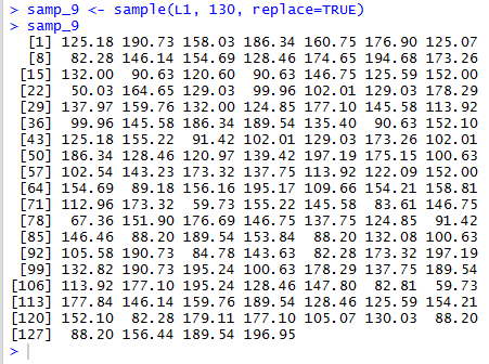
Another feature of sampling with replacement is that we can actually generate a sample that is bigger than the size of our population. The statement samp_9<-sample(L1,130,replace=TRUE) selects 130 random values from the 98 values in L1. It can do this only because the sampleing is done with replacement. The result is shown in Figure 5.

Figure 5