Real World Data 01

Return to Topics page
We will take a small detour from the main path of the course. So far we have seen multiple uses of the gnrnd4 function to generate data that we can then use in an RStudio session. A reasonable question that may have been in your mind would be "Is gnrnd4 of use beyond this course?" The answer is, "Yes, but only if you are teaching a similar course."

I use gnrnd4 because it allows me to generate different kinds of data based on two or three key values. Furthermore, using those key values, the same data values can be generated on my web page, in your RStudio session, or even on a TI-83/84 calculator by using a version of the gnrnd4 program within the web page, within your RStudio session, or on a TI-83/84 calculator, respectively. All of that means that you as a student, in general, do not have to type in a long list of data and I as an instructor can have you work with data that is more than just of few items long.

In the real world, the data that we want to use, for either descriptive or for inferential statistics, will most likely need to be read into a RStudio session. For example, back in an earlier page, toward the bottom of the page, we were given a revised link to a site that provides financial data for Washtenaw County. Figure 1 shows a part of that page.

Figure 1

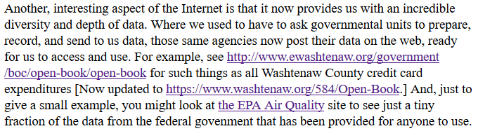
If you click the link on that page, namely, https://www.washtenaw.org/584/Open-Book, you get a new page that contains, among other links, this link to Credit Card Charges:

Figure 1a

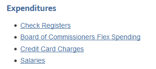
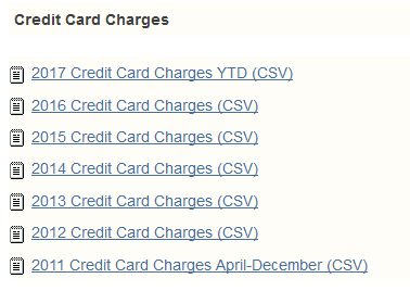
Clicking on the Credit Card Charges takes us to the links shown in Figure 2. This data is provided to anyone who wants it as part of an effort to keep the county's financial records open to the public. We will use the 2015 Credit Card Charges to demonstrate processing "real data" rather than the data that we get in this course by using gnrnd4.

This demonstration is meant just to broaden your view of what can be done. Even though the data in the file is in pretty good shape we will have to do a few slightly fancy things in order to really use it. In doing so, we will be seeing (not learning) extra features of the R language. This course is intended to teach the essentials of statistics. It is not intended to teach any more about R than you need to know in order to support learning those basics of statistics. Therefore, it makes much more sense to limit ourselves to the data produced by gnrnd4 and to leave really learning R to a course designed and advertised to teach R. In particular, you are not expected to be able to read data from a file as part of this course.

Figure 2

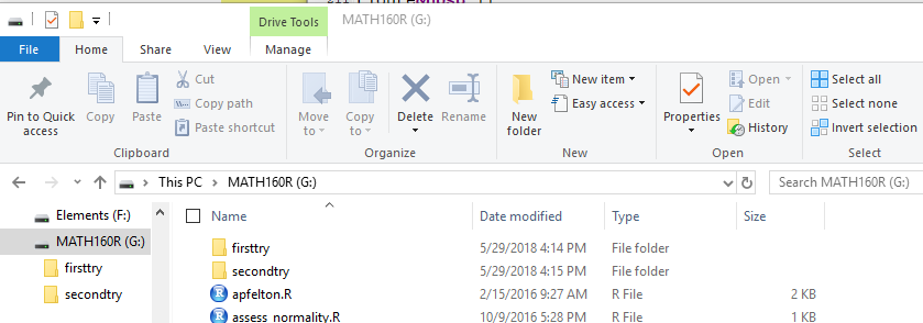
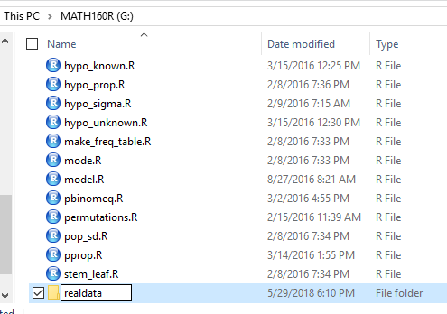
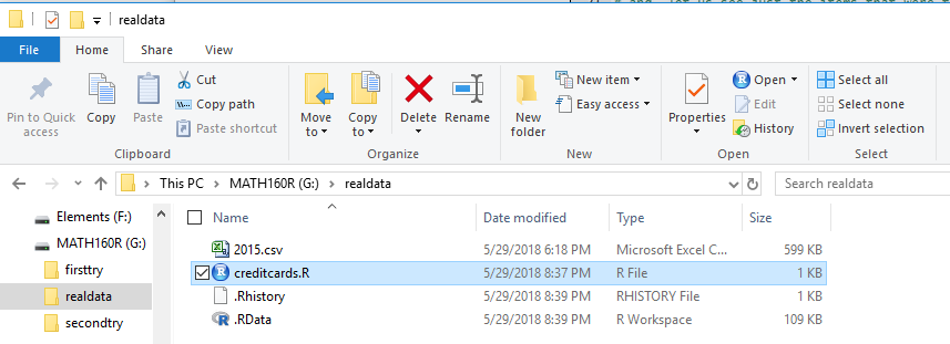
We will start our work, as usual, inserting our USB drive. Part of the display of the contents of my drive is shown in Figure 3.

Figure 3

We create a new director and give it an appropriate name, I chose realdata, as shown in Figure 4.

Figure 4

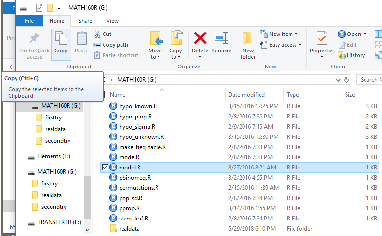
Then we make a copy of model.R.

Figure 5

Next we move to the newly created directory and take the step needed to tell the computer to paste a copy of the file into the currently empty directory.

Figure 6

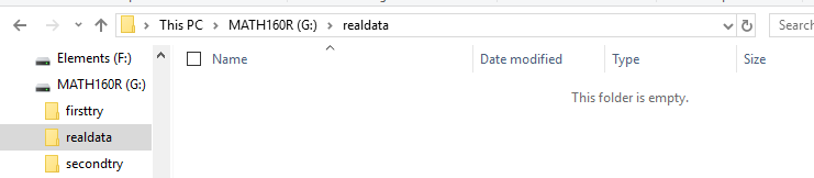
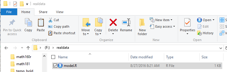
Figure 7 shows the new model.R file in our new directory.

Figure 7

Then we can return to the web page shown back in Figure 2. There our interest is the link for 2015 Credit Card Charges shown in Figure 8.

Figure 8

Click on that link. On my web browser, with my settings, that opened the window shown in Figure 9. [With different browsers and different settings and on different computers other actions may need to be take. Our goal is to have the browser download the file into our newly created directory on the USB drive. Figures 9 through 13 here record the process as it played out on my computer.]

Figure 9

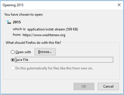
Since the setting to Save File was already checked, I just clicked on the OK. This brings up the screen shown in Figure 10.

Figure 10

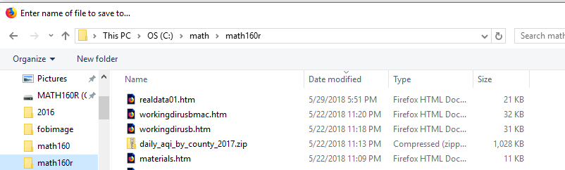
Figure 10 shows that the system is tryong to save the file in the C: dirive. I do not want to save it there, so I click on the MATH160R drive. On my machine this brought up the screen shown in Figure 11.

Figure 11

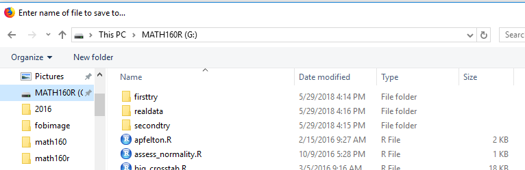
Now, in Figure 11, the file woud be saved on the USB drive. But I want it saved in the realdata folder. Therefore, I clisk on that folder, to bring up Figure 12.

Figure 12

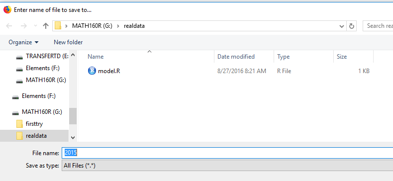
Figure 12 shows us that the file would be saved in the desired directory. However, there is no file extension on the name of the file. I want the file to end with the .csv extension. Therefore, in Figure 13 I have added that extension.

Figure 13

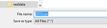
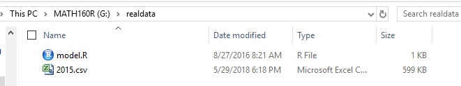
Then we click on the Save button. Once the download is complete we should see, in our new folder, two files. This is shown in Figure 14. You might note that our dta file is relatively large at 599 KB. As we will see later, this is not the sort of data that we would want to enter by hand.

Figure 14

Just so that we can look at the contents of the file we can point to it and left click to open the left pane in Figure 15. There we point to the Open with option to open the pane that allows us to choose the program to use.

Figure 15

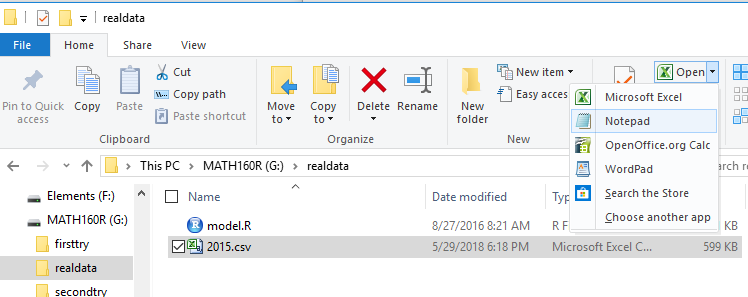
We click on the Notepad option to use that standard text editor. This will start that program which will then display the contents of the file, the start of which is shown in Figure 16.

Figure 16

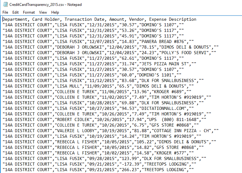
We look at the data so that we can see its organization and some of the values. In Figure 16 we see that there is a header line in the file, a line that gives the titles of the fields in each of the subsequent data lines. There are six (6) different header values. The fourth value is Amount. Following that header line, we see the first number of data lines. In this file, commas are used to separate data. This makes this a csv, comma separated data file. The fourth value on each line corresponds to the Amount of the charge. Reading the first data line shows us that there was a charge of $30.57 on 12/31/15, probably for pizza. We see that there are six (6) data values in each data line.

Once we have seen some of the data we can close that window (end the Notepad program) and return to the view of our directory. There, in Figure 17, we have changed the name of our R script file from model.R to creditcards.R, just to be more meaningful.

Figure 17

Once that is done we can double click on the file to open the RStudio session shown in Figure 18.

Figure 18

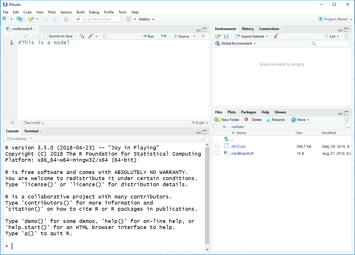
For this demonstration we will use a pattern of

composing our commands in the Editor pane
highlighting the commands that we want to run
using the to have RStudio perform the command in the Console pane
examining the results in the Console pane

We use this pattern so that we can save the commands of the complete session in case we want to perform them again, or if want to publish them or send them to someone else so that they could perform those commands.

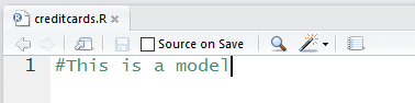
The initial contents of the file show up in Figure 19.

Figure 19

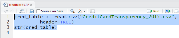
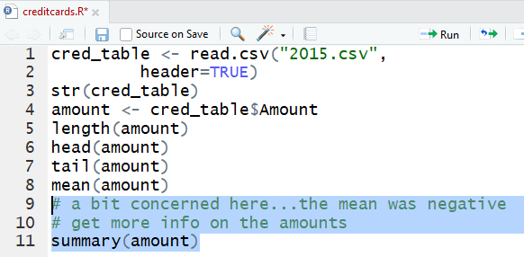
We have changed those to the two commands that we will use to first read the data file (the command will read the file and put the values read into the variable cred_table) and then look at the structure of the resulting cred_table. The lines that we use are:

cred_table <- read.csv("2015.csv",
         header=TRUE)
str(cred_table)

as shown in Figure 20. The read.csv command will instruct R to read a comma separated file named CreditCardTransparency_2015.csv from the current working directory and that the file has a header line. [This is again part of the beauty of confining our work to our newly created directory. We put the data file here and now we do not need to search to find it.]

Figure 20

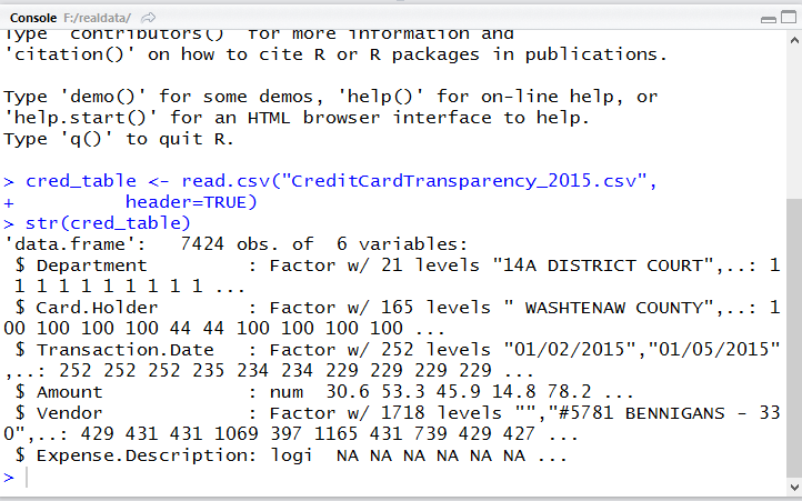
After running the highlighted commands of Figure 20 we see the result in the Console pane shown in Figure 21. There we see that the actual read.csv statement produced no output response, but the str gave us numerous lines that say, among other things, that cred_table is a data.frame with 7424 observations (i.e., rows) of 6 different variables. The variables correspond to the six different values that we saw in each line of the data file back in Figure 16. The output continues with a description of each of the variables,

$Department, $Card.Holder, $Transaction.Date, $Amount,
$Vendor,

and $Expense.Description. Of those, the one we are interested in is the $Amount. We see the first few values of that variable are 30.6, 53.3, 45.9, 14.8, and 78.2. We know that these are rounded values because back in Figure 16 we saw that the actual values are 30.57, 53,26, 45.91, 14.83, and 78.15.

Figure 21

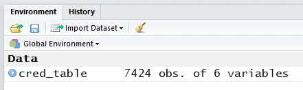
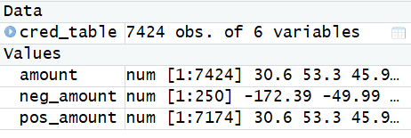
If we look at the Environment pane, shown in Figure 22, we see the report that really tells us that we have a data frame called cred_table defined.

Figure 22

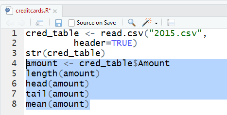
We return to the Editor pane and add the commands

amount <- cred_table$Amount
length(amount)
head(amount)
tail(amount)
mean(amount)

The first one makes a copy of the 7424 $Amount values and puts that copy into a variable called amount. This is just a bit of laziness so that it is easier to refer to the values. Then we confirm the length of amount, look at the first few and then the last few items in amount, and finally, compute the mean of those values.

Figure 23

The commands, highlighted in Figure 23, are run to produce the output seen in Figure 24.

Figure 24

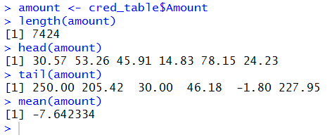
The output looks good, at least up to the point where we find that the mean is a negative value. How can the mean charges be negative?

Just looking at the values shown in Figure 24 as the result of the tail(amount) command, we see that there is at least one such negative value. We might conjecture that negative values represent corrections, refunds, or perhaps something else. Let us see a bit more.

We add the commands

# a bit concerned here...the mean was negative
# get more info on the amounts
summary(amount)

to the editor pane.

Figure 25

Perform those lines.

Figure 26

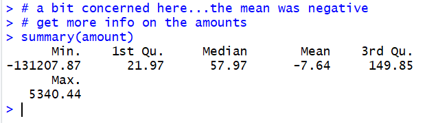
Hold on! The most negative charge was for -$131,200. Perhaps that was a payment against the credit card account? To really go further we would need to either find some more documentation about the values in the file (perhaps there was some explanation page on the web site) or we could call the county and ask about this. Such confusion and uncertainty is quite common in data files that we did not make ourselves. This is an important lesson for us. Be careful to inspect the data!

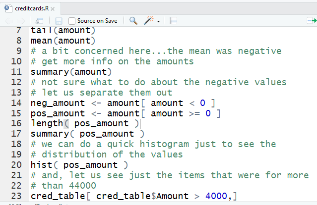
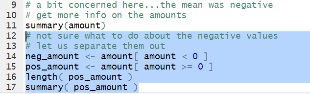
Even with this uncertainty, we want to at least do a bit more work here. Let us add some new commands to the Editor pane.

# not sure what to do about the negative values
# let us separate them out
neg_amount <- amount[ amount < 0 ]
pos_amount <- amount[ amount >= 0 ]
length( pos_amount )
summary( pos_amount )

These may seem a bit strange as statements. If this were a course in R programming, we would want to explain them and learn them. For this course we will just accept them as working statements.

Figure 27

The first command neg_amount - amount[ amount < 0 ] is really wasted. We did not need it and we did not use the results. The second command just pulls out all of the non-negative values from amount and puts them into a new variable called pos_amount. Then we can look at just those non-negative values. We see the result in Figure 28.

Figure 28

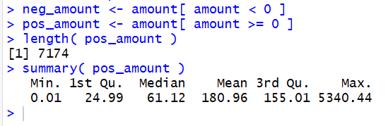
For the non-negative values we see that there are 7174 such values, the vast majority of the original 7424 lines of data. Furthermore, they range from $0.01 to $5,340.00, with a mean value of $181.00 and a median value of $61.12, so there are half the charges for less and half for more than that median amount.

A quick look at the Environment pane, Figure 29, shows the variables that have been created in our workspace.

Figure 29

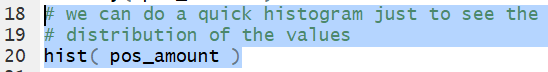
We might as well ask R to do a quick histogram of the data. We add new lines to the Editor pane.

# we can do a quick histogram just to see the
# distribution of the values
hist( pos_amount )

Figure 30

When we run that we get a plot similar to that shown in Figure 31. (The plot that we get depends upon the size of our screen, our RStudio window, and of the Plots pane.)

Figure 31

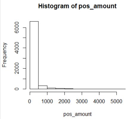
Nothing out of the ordinary in the plot, but it is nice to see.

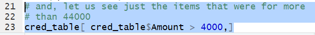
On the other hand, we are a bit curious about the largest charges. To look at this we will return to our data frame because it has all of the information in it. We will construct a command to display the information about all charges that are for more than $4,000.00. Again, constructing such a command is beyond the goals of this course. We do it here just as an example. The command lines are

# and, let us see just the items that were for more
# than 44000
cred_table[ cred_table$Amount > 4000,]

Figure 32

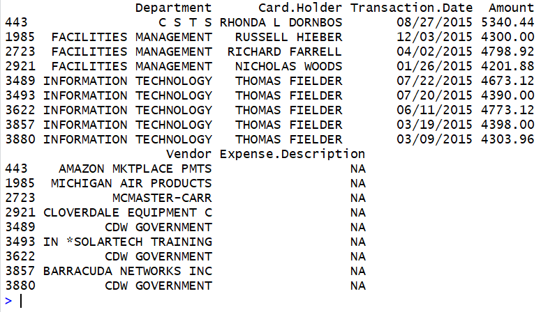
The resulting output is shown in Figure 33. Note that the output has been split into two sections because each line of output contains six values and there is no room in our Console pane to show all that information in one line reading left to right. Therefore, the output shows the first three values for each of the nine (9) instances found with charges over $4000.00, followed by the remaining three values for each of those nine (9) instances.

Figure 33

That is all very interesting, and perhaps it raises some questions, perhaps it leads us to more investigations. But not now.

Before we leave we should return to the Editor pane and click on the

icon to save the file we have created. Figure 34 shows that we have done this so the name of the file, creditcards.R, appears in black.

Figure 34

Then, in the Console pane, we terminate our session as usual.

Figure 35

This brings us back to the view of the directory that we have created for this demonstration. In Figure 36, because this was done on a PC and not on a Mac, we can see the hidden files. In particular, we note that the .RData file, the one that holds the workspace, is quite large, 109 KB. Recall that it holds the entire data frame, the copy of the $Amount that we made in amount, and then a second copy of all of that broken into two parts, neg_amount and pos_amount.

Figure 36