Reading Normal Distribution Tables

Virtually every text on statistics includes an appendix full of tables. One of those tables is sure to give the cumulative frequency of the normal distribution. Although it might seem reasonable to have a standard presentation of such a table, this is not the case. For the cumulative frequency of a normal distribution most tables have some way to associate a z-score with a table value.

A common approach to this is the "cross-table" arrangement. Here we break the z-score into two parts, the left part is usually the units and tenths digits and the right part is the hundredths digit. Thus, a z-score of 2.41 becomes 2.4 and 0.01. Then we use the left part to identify a row of the table and the right part to identify a column of the table. The table item at the intersection of the row and column is the desired table value for that combined z-score.

Here is a typical portion of such a table. (Note that the z-score we are to look up in the table changes every time this page is loaded.)

An alternative arrangement, the list arrangement, gives the possible z-scores along with the table associated value. In order to conserve space, this list of pairs of values is given in multiple columns. Here is a typical portion of such a table. (Note that the z-score we are to look up in the table changes every time this page is loaded, but it is the same as in the example above.)

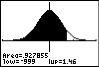
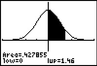
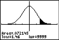
As if having the two different arrangements, the cross and list arrangements, is not difficult enough, various tables provide values representing different areas under the normal curve. As a result, in order to coorrectly interpret the table values we need to understand what the values in the tables represent. Thus for a given z-score, let us take 1.46, different tables may prseent the area under the normal distribution curve from

negative infinity to 1.46,
0 to 1.46,
1.46 to positive infinity.

Using graphs we could represent this by the shaded areas in

negative infinity to 1.46	0 to 1.46	1.46 to positive infinity
To find P(x<1.46) the graph and table give it directly.	To find P(x<1.46) the graph and table are missing the first half of the area so we need to add 0.5 to the table value.	To find P(x<1.46) the graph and table give the part we do not want so we need to subtract the table value from 1.000.
To find P(x>1.46) the graph and table give the part we do not want so we need to subtract the table value from 1.000.	To find P(x>1.46) we want just the part to the right of the shaded area. We get this by taking 0.5000 and subtracting the to the table value.	To find P(x>1.46) the graph and table give it directly.
To find P(x<^–1.46) we use the symmetry of the distribution to realize that P(x<^–1.46)=1.000 – P(x<1.46). Therefore we take 1.000 minus the table value.	To find P(x<^–1.46) we use the symmetry of the distribution to realize that P(x<^–1.46)=1.000 – P(x<1.46). Because the table value is only giving us the portion greater than 0, we take 0.500 minus the table value.	To find P(x<^–1.46) we use the symmetry of the distribution to realize that P(x<^–1.46)=P(x>1.46). Therefore we just take the table value.

One way to ease some of the pain in using the "negative infinity to 1.46" style table is to have that table have z-scores that include negative values.

Here are links to four different web presentations of the cumulative normal distribution. These different pages illustrate some of the differences noted above.