abline()
abline() is used to draw lines on a
plot that has been created. In this course there is no requirement to use this function.
However, it does appear in many examples as a way to enhance other
graphs. In those cases the web pages go a long way toward providing help using
this function. Here we will look at just one example. The source code is given,
along with comments, so that the code can be copied to an RStudio session.
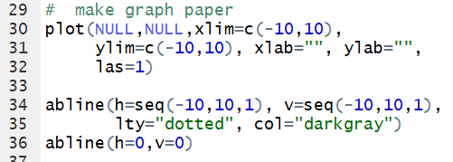
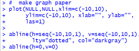
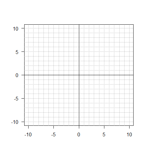
#  make graph paper
plot(NULL,NULL,xlim=c(-10,10),
     ylim=c(-10,10), xlab="", ylab="",
     las=1)

abline(h=seq(-10,10,1), v=seq(-10,10,1),
       lty="dotted", col="darkgray")
abline(h=0,v=0)
Editor view:
 Console view:
Plot:
barplot()
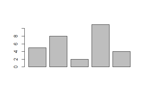
barplot() creates a graph based upon
the values given in the command.
Thus, if we want to have a barplot()
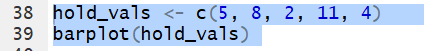
where the bars have a height of 5, 8, 2, 11, and 4 then we can use the commands
hold_vals <- c(5, 8, 2, 11, 4)
and barplot(hold_vals).
Editor view:
 Console view:
Plot:
It is essential to note here that
barplot()
uses its input values to specify the height of each bar.
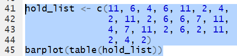
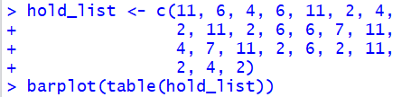
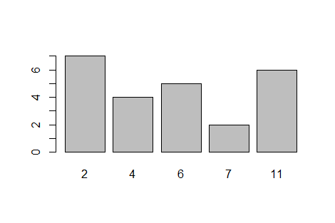
As such, to get bar pot of the frequency of the values in the list
11, 6, 4, 6, 11, 2, 4, 2, 11, 2, 6, 6,
7, 11, 4, 7, 11, 2, 6, 2, 11, 2, 4, and 2 we would first need to get the frequency
of each of the different values in the list.
This could be done by the statements
hold_list <- c(11, 6, 4, 6, 11, 2, 4, 2, 11, 2, 6, 6,
7, 11, 4, 7, 11, 2, 6, 2, 11, 2, 4, 2)
and
barplot(table(hold_list)).
Editor view:
 Console view:
Plot:
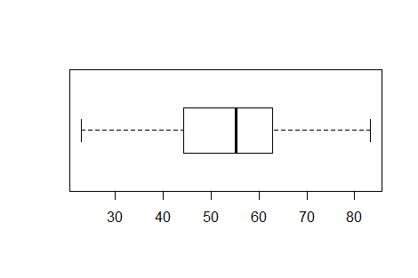
boxplot()
boxplot() uses the list of values given to it
to produce a box and whisker plot.
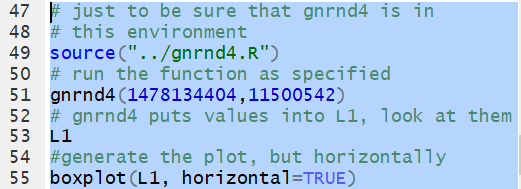
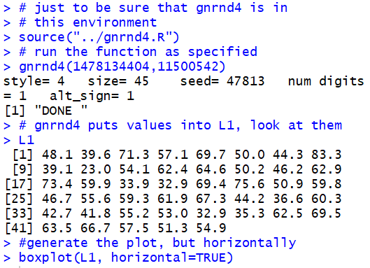
Consider the data in Table BOXPLOT DATA
The function gnrnd4(1478134404,11500542)
will generate the numbers given in the table and put those values into
the variable L1. Then, we can generate the
box and whisker plot via the command boxplit(L1).
However, that command produces a chart with a vertical orientation.
In general, it is easier to use the chart if it has a horizontal
orientation. Therefore, the suggested form of the command
is boxplot(L1,horizontal=TRUE).
Editor view:
 Console view:
Plot:
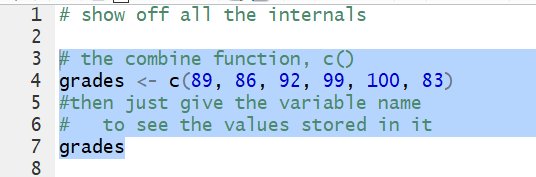
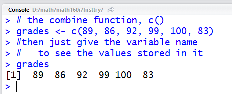
c()
c() function is used to combine values into a single
list. Thus the command grades <- c(89, 86, 92, 99, 100, 83)
puts the values 89, 86, 92, 99, 100, 83 into a variable
called grades.
Editor view:
 Console view:
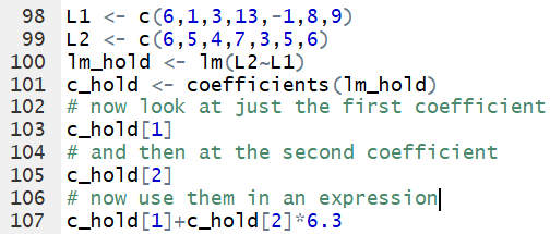
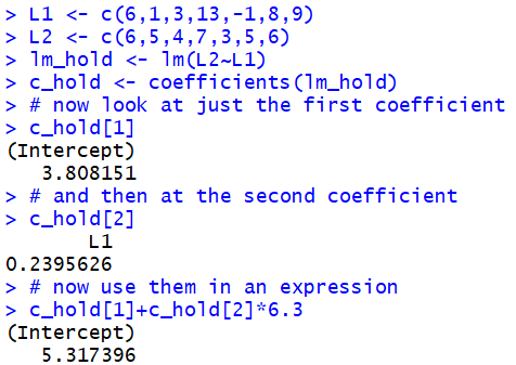
coefficients()
coefficients() function to
extract the coefficients from a linear model.
To see this we will construct such a model and then
use the function on it. For
L1 <- c(6,1,3,13,-1,8,9) and
L2 <- c(6,5,4,7,3,5,6)
we construct and save a linear model via the command
lm_hold <- lm(L2~L1).
Then,we can extract and save the coefficients, that is the
values for a and b in the equation
y = a + bx, via the
command c_hold <- coefficients(lm_hold).
Now, we can look at the first coefficient via the command
c_hold[1] and the second via the command
c_hold[2].
The beauty of this is that we can use those
variables in an expression.
For example, if we wanted to evaluate
a+b*6.3 we can have R do this as
c_hold[1]+c_hold[2]*6.3.
Editor view:
 Console view:
cor()
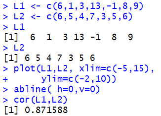
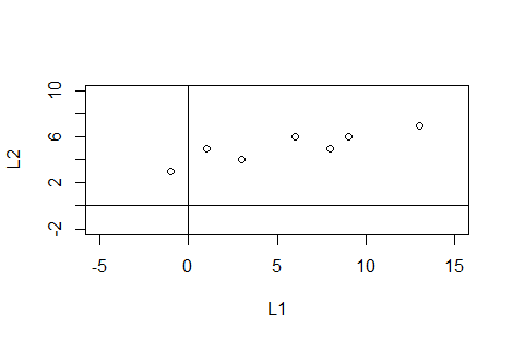
cor() produces the correlation coefficient
for two lists. Thus cor(L1,L2) will generate the correlation coefficient
for the relationship between the values in L1 versus the corresponding values in L2.
In a more traditional mathematics setting, the L1 values represent the x values and the
L2 values represent the y values in ordered pairs of point. For example, for the points
(6,6), (1,5), (3,4), (13,7), (-1,3), (8,5), and (9,6) we could create L1 and L2 via
L1 <- c(6,1,3,13,-1,8,9) and
L2 <- c(6,5,4,7,3,5,6). Then we would use the command
cor(L1,L2) to compute the correlation coefficient for the
relationship.
Editor view:
 Console view:
Plot:
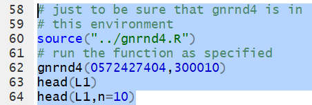
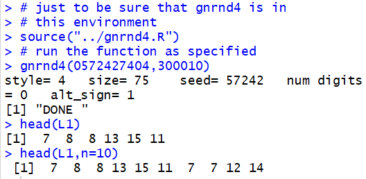
head()
head() function
displays the first items, by default the first 6 items,
in a list of values. Thus, we could use gnrnd4
to generate, in L1, all of the following values.
Then, we could use the command
head(L1)
to have the first items in the list displayed in the console.
To display the first 10 items we add the n=10
argument so the command becomes
head(L1,n=10).
Editor view:
 Console view:
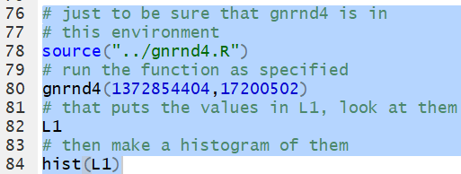
hist()
hist() is used to generate a
histogram of the values that are given to it. Thus, we have
the values shown in Table DATA FOR HISTOGRAM:
The function gnrnd4(1372854404,17175502)
will generate the numbers given in the table and put those values into
the variable L1. Then, we can generate the
histogram for those values via the command
hist(L1).
Editor view:
 Console view:
Plot:
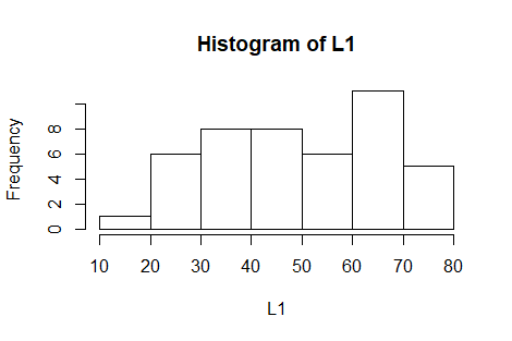
Some note should be made here about the decisions that R has made in creating the histogram. It was R that determined the number of bars to use and the values to use as the breaks for that grouping. Furthermore, the intervals are closed on the right. That means that that the interval holding the value
64.9 is
(60,70], where the closing bracket,
], indicates the value 70, and there is one in our data,
is included in this interval.
You can override these decisions but the commands to do so are beyond the scope
of this page.
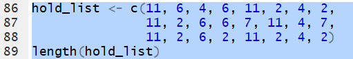
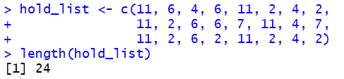
length()
length() produces the number of items in a list.
Thus, we could construct a list via
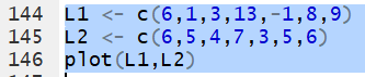
hold_list <- c(11, 6, 4, 6, 11, 2, 4, 2, 11, 2, 6, 6, 7, 11, 4, 7, 11, 2, 6, 2, 11, 2, 4, 2)
and then the command
length(hold_list)
will display the number of items in our list.
Editor view:
 Console view:
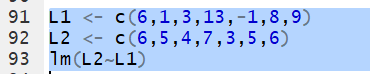
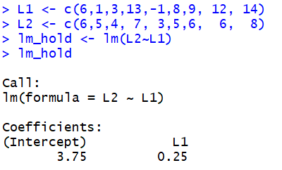
lm()
lm() function
to produce a linear model, that is to do a linear regression,
based on two lists of values.
For the points
(6,6), (1,5), (3,4), (13,7), (-1,3), (8,5), and (9,6) we could create L1 and L2 via
L1 <- c(6,1,3,13,-1,8,9) and
L2 <- c(6,5,4,7,3,5,6).
Here L1 holds the x values and L2
holds the y values. Our goal in getting a linear model is to find values for
a and b in the equation y=a+bx. The a
represents the y-intercept and the b
represents the slope of the regression line. The command to get these two values
is lm(L2~L1). It is essential to note the
order of the two lists. The dependent variable, y, represented by L2 goes first.
The independent variable, x, represented by L1, goes second.
Between the two is the character ~, tilde.
Examine the commands and the console output from those commands.
Editor view:
 Console view:
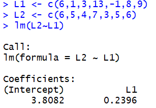
The console view shows us that the value of the intercept, the a in our equation is 3.8082 (rounded to 4 decimal places), and the value of the slope, the b in our equation, is 0.2396. Therefore, our equation reads
y = 3.8082 + 0.2396*x
Our use of the
lm() function, as shown above,
produces the two immediately desired values.
However, most of the time we are better off if we
assign the result of the function to a variable. For example, we could use
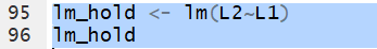
lm_hold <- lm(L2~L1)
and then just use that variable to achieve the same result that we saw above.
Editor view:
 Console view:
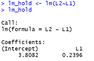
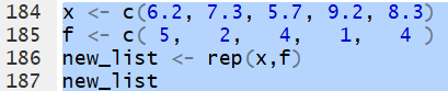
That does not look, so far, like any improvement. However, storing the result of the
lm() function saves much more than is
shown in the console. In fact, if you were to look in the environment
pane you would notice that we have
Environment view:
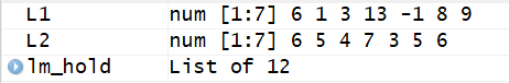
Our variable,
lm_hold, is clearly much more complex than
any other variable we have seen. See the web pages on doing linear regression for
more details on advanced consequences of storing the results of the function in a
separate variable. [Also see coefficients() and
residuals().]
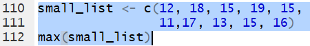
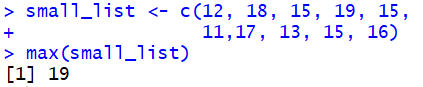
max()
max() finds the largest value in a list.
Thus, for the list defined by
small_list <- c(12, 18, 15,
19, 15, 11,17, 13, 15, 16)
the command max(small_list)
produces the value 19.
Editor view:
 Console view:
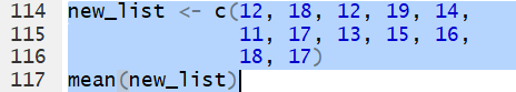
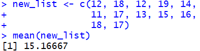
mean()
mean() finds the mean,
the arithmetic average, of the values in the list.
Thus, for the list defined by
new_list <- c(12, 18, 12, 19, 14,
              11, 17, 13, 15, 16,
              18, 17)
the command mean(new_list)
produces the value 15.16667.
Editor view:
 Console view:
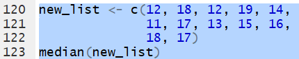
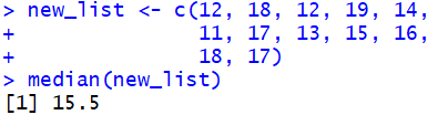
median()
median() finds the median,
the middle (once the list is sorted), of the values in the list.
Thus, for the list defined by
new_list <- c(12, 18, 12, 19, 14,
              11, 17, 13, 15, 16,
              18, 17)
the command median(new_list)
produces the value 15.5.
Editor view:
 Console view:
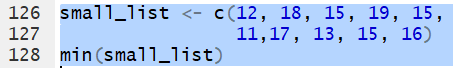
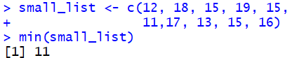
min
min() finds the least value in a list.
Thus, for the list defined by
small_list <- c(12, 18, 15,
19, 15, 11,17, 13, 15, 16)
the command min(small_list)
produces the value 11.
Editor view:
 Console view:
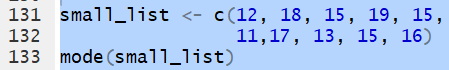
mode()
mode() function is
incuded here not so much for what it does as for what it does not do.
In particular, the mode() function does
NOT find the mode of a list of values. Rather, mode()
just reports the kind ofvalue stored in a variable name. [In order to find the
mode of a list of values you can use the Mode()
function, note the capital M, that is provided both on the
USB drive and on my web site.] If we have a list of values, for example
small_list <- c(12, 18, 15,
19, 15, 11,17, 13, 15, 16)
then the command mode(small_list) produces
the text "numeric" to tell us that the list is holding
numeric values.
Editor view:
 Console view:
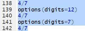
options()
options() function is used to change
the setting of various system parameters. In this class there is but one such
parameter that we may want to change and that is the number of digits that
R tries to show for values. The default number is 7. We can see this if we
try to use R to find the value of 4/7,
which R displays as 0.5714286.
We can increase the number of digits to display via the command
options(digits=12).
Then, if we perform the same division we get
0.571428571429.
Of course we could reset the default via
options(digits=7).
Editor view:
 Console view:
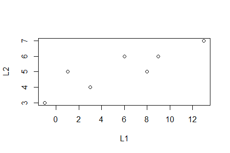
plot()
plot() function creates a
scatter graph for points represented by the values in two parallel lists.
For the points
(6,6), (1,5), (3,4), (13,7), (-1,3), (8,5), and (9,6) we could create L1 and L2 via
L1 <- c(6,1,3,13,-1,8,9) and
L2 <- c(6,5,4,7,3,5,6).
Then we would use the command
plot(L1,L2) to
create a rough plot of the values.
Editor view:
 Console view:
Plot:
There are many additional arguments that can be specified to change the appearance of the plot and we can add certain lines to the plot via the
abline() function. This
page was never intended to teach and/or explain these other options, but we can
at least look at a more complete statement. We will look at the following
commands
plot(L1,L2,
     main="Demonstration of plot()",
     xlim=c(-6,16), ylim=c(-6,10),
     pch=16, las=1, xaxp=c(-6,16,11),
     yaxp=c(-6,10,8), cex.axis=0.7,
     xlab="x values", ylab="y values")
abline( h=seq(-6,10,2), v=seq(-6,16,2),
        col="darkgray",
        lty="dotted")
abline(h=0,v=0,col="blue")
These produce the following graph.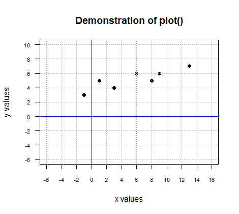
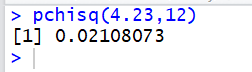
pchisq()
pchisq() gives the area,
for the χ² distribution, to the left of the value
x for a given degrees of freedom,
df. Thus, the usual form of the
command is
pchisq( x, df ). For example,
the area to the left of 4.23 for 12 degrees of freedom is written as
pchisq(4.23,12).
Editor view:
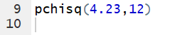 Console view:
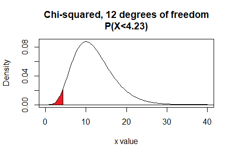
Here is a plot of that area, generated apart from the commands shown above.
Plot:
pchisq() also allows the use of the
lower.tail=FALSE argument to change the meaning
of the function so that it gives the area to the right of the specified value.
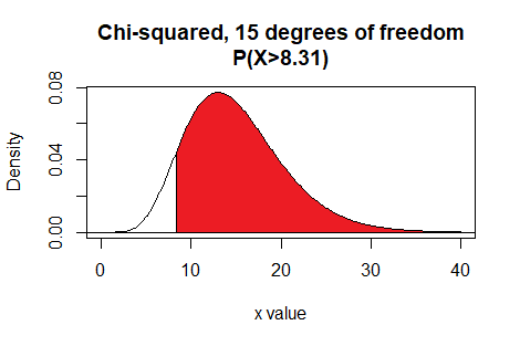
Thus the command pchisq(8.31,15,lower.tail=FALSE)
gives the area under the curve to the right of
8.31 with 15 degrees of freedom.
Editor view:
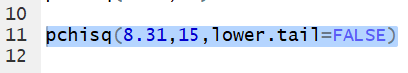 Console view:
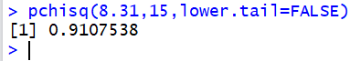
Here is a plot of that area, generated apart from the commands shown above.
Plot:
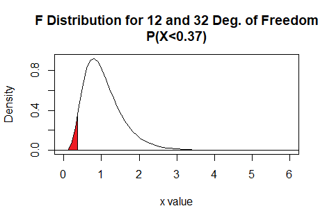
pf()
pf() gives the area,
for the F distribution, to the left of the value
x for two given degrees of freedom,
df1 and
df2. Thus, the usual form of the
command is
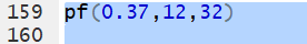
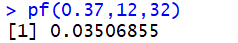
pf( x, df1, df2). For example,
the area to the left of 0.37 for 12 and 32 degrees of freedom is written as
pf(0.37,12,32).
Editor view:
 Console view:
Here is a plot of that area, generated apart from the commands shown above.
Plot:
pf() also allows the use of the
lower.tail=FALSE argument to change the meaning
of the function so that it gives the area to the right of the specified value.
Thus the command pf(1.78,32,12,lower.tail=FALSE)
gives the area under the curve to the right of
1.78 with 32 and 12 degrees of freedom.
Editor view:
 Console view:
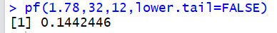
Here is a plot of that area, generated apart from the commands shown above.
Plot:
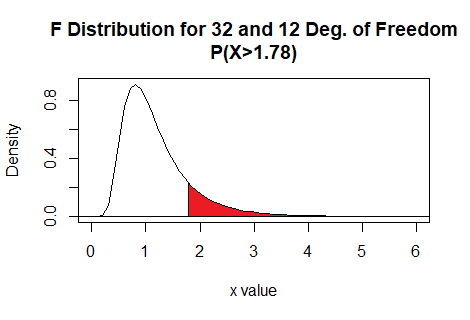
pnorm() pnorm() function gives the
area, under the normal distribution curve, to the left of a specified
value. Thus, the command
pnorm(-0.83) gives the area to the left
of -0.83, representing the
probability of getting a value less than -0.83.
Editor view:
 Console view:
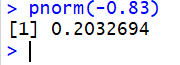
Here is a plot of that area, generated apart from the commands shown above.
Plot:
pnorm() also allows the use of the
lower.tail=FALSE argument to change the meaning
of the function so that it gives the area to the right of the specified value.
Thus the command pnorm(1.68,lower.tail=FALSE)
gives the area under the standard normal curve to the right of
1.68.
Editor view:
 Console view:
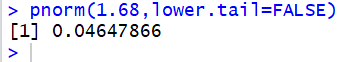
Here is a plot of that area, generated apart from the commands shown above.
Plot:
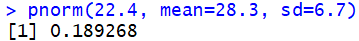
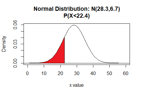
Furthermore,
pnorm() allows us to specify
the mean and/or the standard deviation of the distribution.
If not specified then the default value is mean=0 and sd=1,
giving the standard normal distribution seen above. For example,
the command
pnorm(22.4, mean=28.3, sd=6.7)
finds the probability of getting a value less than 22.4 in a
distribution that is N(28.3,6.7).
Editor view:
 Console view:
Here is a plot of that area, generated apart from the commands shown above.
Plot:
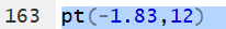
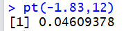
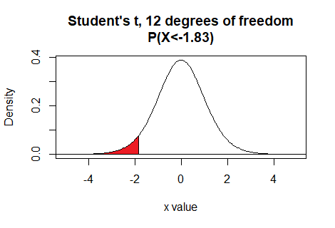
pt()
pt() gives the area,
for the Student's t distribution, to the left of the value
x for a given degrees of freedom,
df. Thus, the usual form of the
command is
pt( x, df ). For example,
the area to the left of -1.83 for 12 degrees of freedom is written as
pt(-1.83,12).
Editor view:
 Console view:
Here is a plot of that area, generated apart from the commands shown above.
Plot:
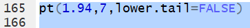
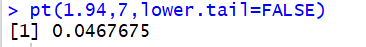
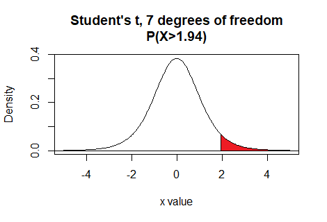
pt() also allows the use of the
lower.tail=FALSE argument to change the meaning
of the function so that it gives the area to the right of the specified value.
Thus the command pt(1.94,7,lower.tail=FALSE)
gives the area under the curve to the right of
1.94 with 7 degrees of freedom.
Editor view:
 Console view:
Here is a plot of that area, generated apart from the commands shown above.
Plot:
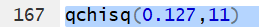
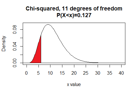
qchisq
qchisq function to give us the
x value that has a given area under the chi-squared curve to the left of that x
value. This is done for a specific number of degrees of freedom.
Therefore, the general form of the command is
qchisq(area,df) where the
area is the desired probability to the left, and
df is the degrees of freedom.
Thus, for 11 degrees of freedom, if we want to
find the x value that has 12.7% of the area
to the left of that value then we just need to use the command
qchisq(0.127,11)
Editor view:
 Console view:
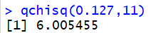
This tells us that for 11 degrees of freedom, the area to the eft of
6.005455 is 0.127.
Here is a plot of that area, generated apart from the commands shown above.Plot:
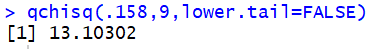
qchisq() also allows the use of the
lower.tail=FALSE argument to change the meaning
of the function so that it uses the area to the right of the desired value.
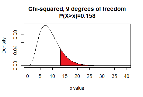
Thus the command qchisq(.158,9,lower.tail=FALSE)
gives the x value that has 15.8% of the
area under the curve to the right of
x with 9 degrees of freedom.
Editor view:
 Console view:
Here is a plot of that area, generated apart from the commands shown above.
Plot:
qf()
qf function to give us the
x value that has a given area under the F distribution curve to the left of that x
value. This is done for a specific pair of degrees of freedom values.
Therefore, the general form of the command is
qf(area,df1,df2) where the
area is the desired probability to the left, and
df1 and df2
are the degrees of freedom.
Thus, for 13 and 42 degrees of freedom, if we want to
find the x value that has 12.5% of the area
to the left of that value then we just need to use the command
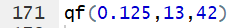
qf(0.125,13,42)
Editor view:
 Console view:
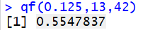
This tells us that for 13 and 42 degrees of freedom, the area to the left of
0.5547837 is 0.125.
Here is a plot of that area, generated apart from the commands shown above.Plot:
qf() also allows the use of the
lower.tail=FALSE argument to change the meaning
of the function so that it uses the area to the right of the desired value.
Thus the command qf(.2,37,8,lower.tail=FALSE)
gives the x value that has 20% of the
area under the curve to the right of
x with 37 and 8 degrees of freedom.
Editor view:
 Console view:
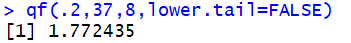
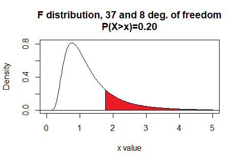
Here is a plot of that area, generated apart from the commands shown above.
Plot:
qnorm()
qnorm() function produces the z value that
is needed to have a given area under the standard normal curve to the left of that
z value. If we want to know the z value that has 0.214 as the area to its left
under the standard normal curve then we use the command
qnorm(0.214). The result of that command is
-0.7926187, therefore,
the P(X<-0.7926187)=0.214.
Editor view:
 Console view:
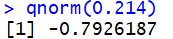
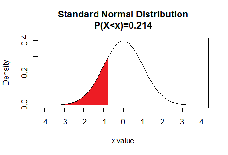
Here is a plot of that area, generated apart from the commands shown above.
Plot:
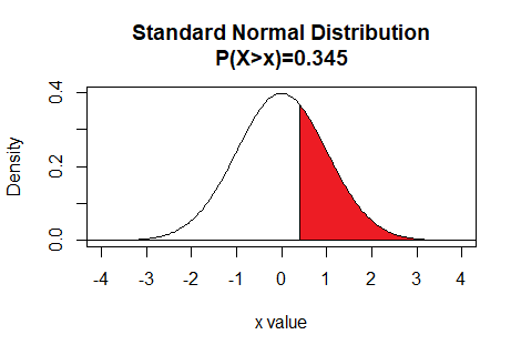
qnorm() also allows the use of the
lower.tail=FALSE argument to change the meaning
of the function so that it uses the area to the right of the desired value.
Thus the command qnorm(0.345,lower.tail=FALSE)
gives the z value that has 34.5% of the
area under the curve to the right of
z.
Editor view:
 Console view:
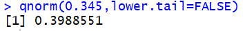
Here is a plot of that area, generated apart from the commands shown above.
Plot:
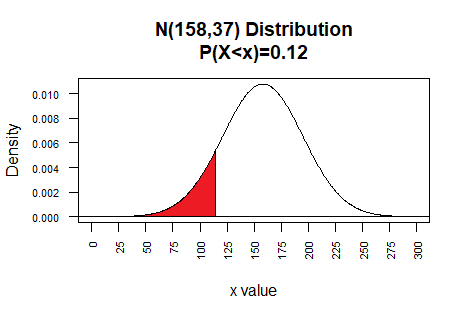
The examples above work for a standard normal distribution. However,
qnorm() also allows the user to specify
the mean and standard deviation of the population. Thus, for a population that
is N(158,37) we can find the value that has 12% of the area
under that curve to the left of that value by using the command
qnorm(0.12,mean=158,sd=37).
Editor view:
 Console view:
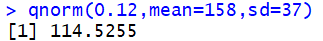
Here is a plot of that area, generated apart from the commands shown above.
Plot:
qt()
qt function to give us the
t value that has a given area under the Student's t curve to the left of that t
value. This is done for a specific number of degrees of freedom.
Therefore, the general form of the command is
qt(area,df) where the
area is the desired probability to the left, and
df is the degrees of freedom.
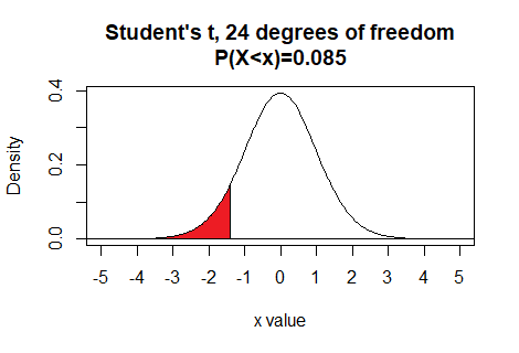
Thus, for 24 degrees of freedom, if we want to
find the x value that has 8.5% of the area
to the left of that value then we just need to use the command
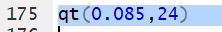
qt(0.085,24)
Editor view:
 Console view:
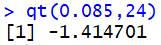
This tells us that for 24 degrees of freedom, the area to the left of
-1.414701 is 0.085.
Here is a plot of that area, generated apart from the commands shown above.Plot:
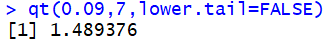
qt() also allows the use of the
lower.tail=FALSE argument to change the meaning
of the function so that it uses the area to the right of the desired value.
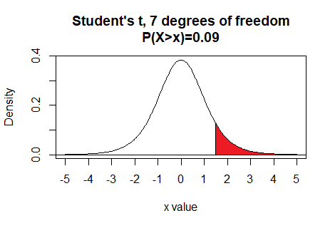
Thus the command qt(0.09,7,lower.tail=FALSE)
gives the t value that has 9% of the
area under the curve to the right of
t with 7 degrees of freedom.
Editor view:
 Console view:
Here is a plot of that area, generated apart from the commands shown above.
Plot:
rep()
rep() function to create a
list
that is made up of different values, each repeated some number of times,
especially where the different values may be repeated a differeent number of times.
Consider the case where we want a list that has the value 6.2 repeated 5 times,
the value 7.3 repeated 2 times, the value 5.7 repeated 4 times,
the value 9.2 just 1 time, and the value 8.3 repeated 4 times.
We can accomplish this with the commands
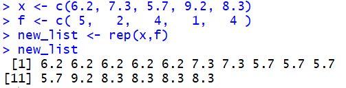
x <- c(6.2, 7.3, 5.7, 9.2, 8.3)
f <- c( 5,   2,   4,   1,   4 )
new_list <- rep(x,f)
new_list
Editor view:
 Console view:
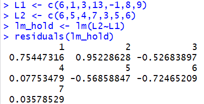
residuals()
residuals() function to
extract the residual values from a linear model.
To see this we will construct such a model and then
use the function on it. For
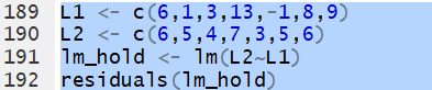
L1 <- c(6,1,3,13,-1,8,9) and
L2 <- c(6,5,4,7,3,5,6)
we construct and save a linear model via the command
lm_hold <- lm(L2~L1).
Then,we can extract and display the residuals via the
command residuals(lm_hold).
Editor view:
 Console view:
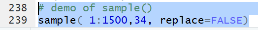
sample()
sample() gets item numbers from a range of integers
to represent a sample of a given size with or without (the default) replacement. Thus
the statement
sample(1:1500, 34, replace=FALSE)
produces a list of 34 distinct values in the range of 1 to 1500.
The values are distinct because the sampling is done without replacement.
Editor view:
 Console view:
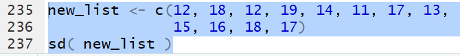
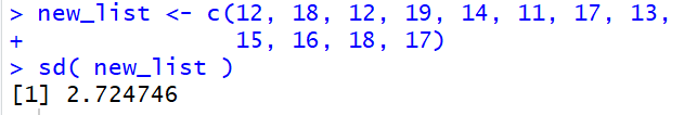
sd()
sd() finds the standard deviation,
of the values in the list assuming that those values reresent a sample rather than a population.
Thus, for the list defined by
new_list <- c(12, 18, 12, 19, 14,
              11, 17, 13, 15, 16,
              18, 17)
the command sd(new_list)
produces the value 2.724746.
Editor view:
 Console view:
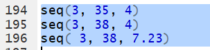
seq()
seq() function to create a
list
that is made up of different values that fall into a nice pattern.
The seq() has a number of different forms, but in this
class it is enough to know the form that
allows you to specify a starting value, a limiting value, and the size of the step that
the pattern of values will take. Thus, we can generate the list 3, 7, 11,
15, 19, 23, 27, 31, and 35 with the command
seq(3,35,4) which means
start at 3,
do not go over 35, but go up in steps
of 4 Note that the
command seq(3,38,4) would generate the same set of numbers.
The second argument expresses a limit to the sequence, not the final value.
Starting at 3 and taking steps of 4 we get to 35 and then we need to stop
because the next value would be 39 and that is over the limit of 38.
Also note that we do not need to use "nice" values.
we can do such things as make the step be 7.23 by
using the command seq(3,38,7.3).
Editor view:
 Console view:
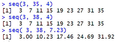
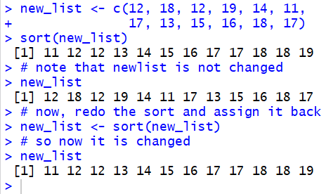
sort()
sort() produces a sorted copy of the list
it is given. It does not, by itself, change the original list. To do that just assign
the sorted list back to the original variable holding the list.
Thus, for the list
new_list <- c(12, 18, 12, 19, 14, 11,
17, 13, 15, 16, 18, 17)
the command
sort(new_list) creates a sorted version of
the list, but it does not change the list.
On the other hand, the statement
new_list <- sort(new_list)
sorts the list and then assigns the sorted list
back to the variable new_list.
Editor view:
 Console view:
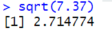
sqrt()
sqrt() function produces the
sqruare root of a value.
Thus,
sqrt(7.37) produces 2.714774.
Editor view:
 Console view:
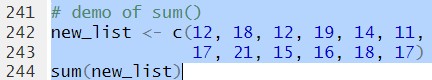
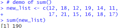
sum()
sum() finds the sum,
of the values in the list.
Thus, for the list defined by
new_list <- c(12, 18, 12, 19, 14,
              11, 17, 13, 15, 16,
              18, 17)
the command sum(new_list)
produces the value 190.
Editor view:
 Console view:
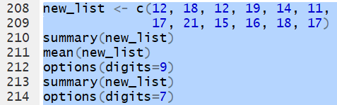
summary()
summary() is used in two different
situations in this course.
First, the summary() of a simple list provides
six (6) differeent descriptive measures for that list. These
are the values for the minimum, the first quartile, the median, the mean, the
third quartile, and the maximum. [Some note should be taen here to point out that there are
a number of different algorithms for finding the 1st and
3rd quartiles and that R uses one that is different
from the one used on the TI-83/84 calculators.]
For the list
new_list <- c(12, 18, 12, 19, 14, 11,
17, 21, 15, 16, 18, 17)
the command
summary(new_list)
gives those values as
11.00, 13.50, 16.50, 15.83, 18.00, and 21.00, respectively.
You may notice that these values have fewer than the default 7 digits displayed.
This is particularly true for the mean where we now that the
mean(new_list) command would produce
15.83333.
This is a good place to change, at least for a moment,
the number of digits to be displayed.
By increasing that number to 9 we can get more digits in our values.
Editor view:
 Console view:
The other use of
summary() is to get a much
more detailed report of the results of a linear regression. We do this by asking for
the summary() of a lienar model.
To see this we will construct such a model and then
use the function on it. For
L1 <- c(6,1,3,13,-1,8,9, 12, 14) and
L2 <- c(6,5,4, 7, 3,5,6, 6, 8)
we construct and save a linear model via the command
lm_hold <- lm(L2~L1).
To merely see the coefficients we just display the linear model
lm_hold.
Editor view:
 Console view:
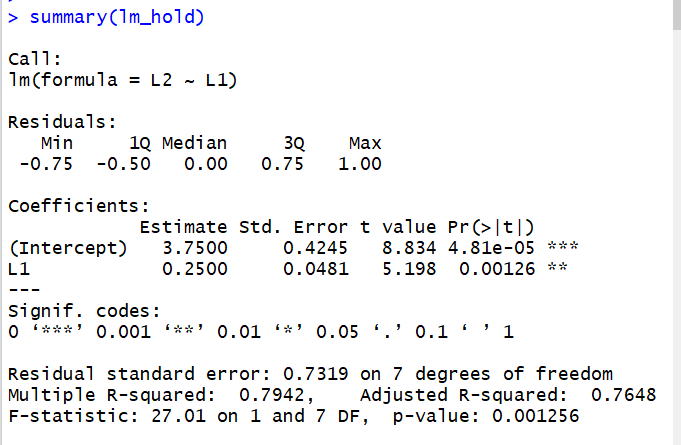
However,the command
summary(lm_hold)
produces that information (in a different format) and much more.
Editor view:
 Console view:
table()
table()
accepts as an argument a list of values. It then
produces a list
that has as its values the frequency of the values in
the original list. Furthermore, each of those frequencies is
given the label that is the value being tallied.
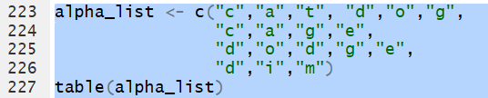
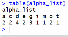
Thus, for the list
alpha_list <- c("c","a","t","d","o","g",
"c","a","g","e",
"d","o","d","g","e",
"d","i","m")
the command table(alpha_list) will hold
the frequency of each letter and those frequencies will have
the label of the letter.
Editor view:
 Console view:
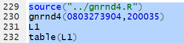
Or, for the values in the following table We can generate those values, inspect them (just to be sure they are right), and then use
table(L1)
to get the frequency of each unique value.
Editor view:
 Console view:
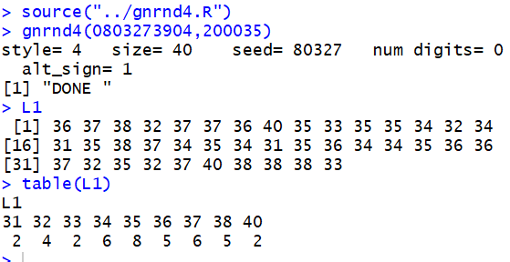
That way we can see, for example, that the value 35 appears 8 times in the table.
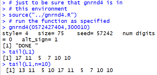
tail()
tail() function
displays the last items, by default the last 6 items,
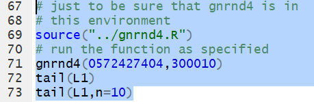
in a list of values. Thus, we could use gnrnd4
to generate, in L1, all of the following values.
Then, we could use the command
tail(L1)
to have the last items in the list displayed in the console.
To display the last 10 items we add the n=10
argument so the command becomes
tail(L1,n=10).
Editor view:
 Console view: