Computing in R: Frequency Tables -- Discrete Values
Return to Topics page
This page presents R
commands related building and interpreting frequency tables for discrete values.
To do this we need some example data.
We will use the values given in Table 1
From the Discussion page we know that we can construct a simple
frequency table for the values in Table 1 as
The question is, how do we do this in R?
Consider the following commands
source( file="http://courses.wccnet.edu/~palay/math160r/gnrnd4.R")
gnrnd4( key1=859459203, key2=800065 )
L1
tabulate(L1)
which we use to generate the data values, verify that we have the same values,
and then attempt to use the R command tabulate() to see if that
produces the desired result.
Figure 1 holds the Console image from an RStudio session
where we performed those commands.
Figure 1
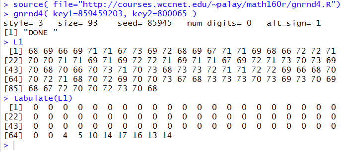
From Figure 1 we see that we have the correct values in the variable L1.
And, looking at the results of the tabulate(L1) command,
we do see the desired values of 4, 5, 10, 14, 17, 16, 13, and 14.
But what are all of those 0's and we know that something happened 4 times, but what value was it that appeared 4 times?
The leading 0's correspond to the number of times that we found 1 in the data (namely 0),
2 in the data (namely 0), 3 in the data (namely 0), and so on.
The final line of the output tells us that both 64 and 65 did not appear in the data, but that 66 appeared 4
time, 67 appeared 5 times, 68 appeared 10 times, and so on.
All of this seems quite messy.
Let us try a different R command, namely table(L1).
Figure 2 shows the result of that command.
Figure 2
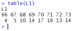
Now that is more like it! The image in Figure 2
is almost identical to Table 2.
We are just missing some identifying text and the lines
to make it look like a table.
To move further with this, we want to be able to look more closely
at the results of the table(L1) command.
Therefore,
we perform the command again,
but this time we save the result in
a variable called freq.
To do this we perform the command freq <- table( L1 ).
Figure 3
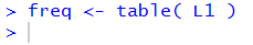 As you can see, in Figure 3, the line that we executed produced no output.
(By the way, getting no output also means getting no
error or warning messages, an indication that everything is OK.)
As you can see, in Figure 3, the line that we executed produced no output.
(By the way, getting no output also means getting no
error or warning messages, an indication that everything is OK.)
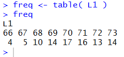
If, however, we now just give the name of the variable, freq,
R displays the contents of the variable, as in Figure 4.
Figure 4
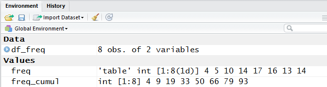
 We could have just looked at the Environment pane of our RStudio
to see that freq is now defined. That is shown in Figure 5.
We could have just looked at the Environment pane of our RStudio
to see that freq is now defined. That is shown in Figure 5.
Figure 5
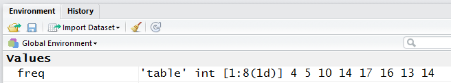 Notice, in the Environment pane, that freq is defined as a 'table'
of integer values, indexed from 1 to 8 as a 1 dimensional structure with values
4, 5, 10, 14, 17, 16, 13, and 14.
There is nothing in the Environment pane to indicated that there are
labels attached to those values.
However, looking back at Figure 4, we see that there clearly are such labels.
Notice, in the Environment pane, that freq is defined as a 'table'
of integer values, indexed from 1 to 8 as a 1 dimensional structure with values
4, 5, 10, 14, 17, 16, 13, and 14.
There is nothing in the Environment pane to indicated that there are
labels attached to those values.
However, looking back at Figure 4, we see that there clearly are such labels.
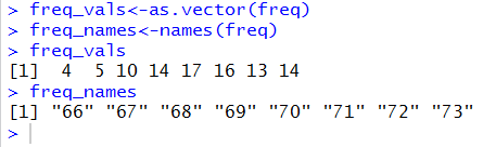
To demonstrate this, and to prepare for the next steps, we
separate those values and labels in freq.
The function as.vector(freq) produces just the list of values in freq.
The function names(freq) produces just the list of labels in freq.
Therefore, the commands by just giving the names of the two new variables,
freq_vals<-as.vector(freq)
freq_names<-names(freq)
not only extract those lists but also assign them to freq_vals
and freq_names, respectively.
If we follow thse two commands
by just giving the two variables,
freq_vals
and freq_names, we see what is now assigned to those two variables.
All of this is shown in Figure 6.
Figure 6
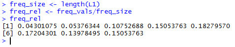
Of course, now that we just have the values stored in freq_vals,
we could find the relative frequency
if we divide that variable by the number of values in L1,
i.e., in Table 1.
We could count those values, but it is much safer to let R
figure this out. The commands
freq_size <- length(L1)
freq_rel <- freq_vals/freq_size
freq_rel
will compute the size of L1, store that value in freq_size,
divide each value in freq_vals by that size, store the
results as values in freq_rel, and finally, display the values in freq_rel.
All of this is shown in Figure 8.
Figure 7
Unfortunately, Table 2 did not include the relative frequency.
We correct that oversight, and prepare for the rest of the work
here by including Table 3.
Our R computed values for the relative frequency shown in
Figure 7 conform to those shown in Table 3.
What about the cumulative frequency? R has a
function, cumsum(), that will create this from the
values stored in freq_vals. Thus the commands
freq_cumul <- cumsum( freq_vals )
freq_cumul
shown in Figure 8, compute the cumulative frequency, store those values in freq_cumul,
and then display those values.
All of this is shown in Figure 8.
Figure 8
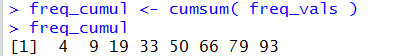
The values shown in Figure 8 match
the cumulative frequency values in Table 3.
The next step is to compute the relative cumulative frequency.
But this is just the cumulative frequency values
divided by the freq_size.
The commands to do this and display the results are
freq_rel_cumul <- freq_cumul/freq_size
freq_rel_cumul
and the use of those commands in R is shown in
Figure 9.
Figure 9
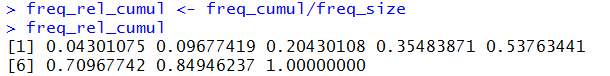
Again, the values shown in Figure 9 correspond to the values in
Table 3 for relative cumulative frequency.
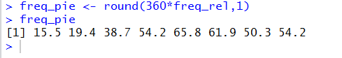
That leaves us with the task
of finding the degrees in a pie chart values shown in Table 3.
To do this we need to multiply 360 times the values in freq_rel,
and we would like to round the result to 1 decimal place.
The R commands to do this and display the results are
freq_pie <- round(360*freq_rel,1)
freq_pie
and the use of those commands in R is shown in
Figure 10.
Figure 10
At this point, in Figures 4, 7, 8, 9, and 10,
we have seen how we can get R to compute all of the values
that we have in Table 3.
It would be nice if we could also get R to
produce a chart such as Table 3
giving all of the values in one place.
However, rather than mimic the horizontal version of the
frequency table shown in Table 3,
we will try to get a version of the vertical
of the frequency table.
Such a vertical version is given as Table 4.
Before we start constructing such a table in R we observe the values
displayed in the Environment pane of our RStudio session.
Figure 11 shows a part of that pane.
Figure 11
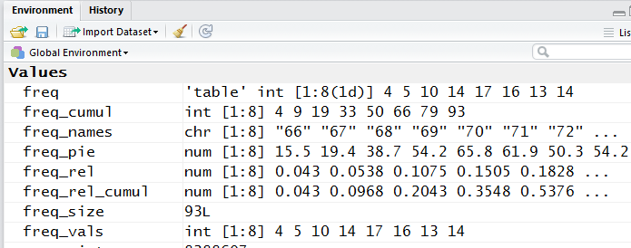
All of the variables shown in Figure 11 are separate entities. We want one entity
that holds many columns of values where each "row" of the entity has related values in it.
Such a structure in R is called a data frame.
We will build that structure from the existing variables.
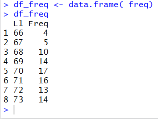
We start with the commands
df_freq <- data.frame( freq)
df_freq
to create a data frame called df_feq from
the table freq. Recall that we know freq
has both labels and values in it. (We saw that back in Figure 6.)
When we perform the commands just noted R
takes the table freq
and puts it into the data frame structure called df_freq.
In doing so, R has created df_freq with two columns,
one for the labels and one for the values.
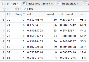
All of this is shown in Figure 12.
Figure 12
The display of df_freq given in Figure 12,
is organized just as we want in order
to mimic Table 4, or at least to start to do this.
The values are arranged in columns.
If we go back to the Environment pane, we see that the variable df_freq
is now defined in the Data area, and that it has 8 observations of
each of two variables. The image of this appears in Figure 13.
Figure 13
R has an additional command View()
that improves upon the display of df_freq.
[Note that View() starts with a capital letter V.]
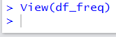
Performing View(df_freq) in the Console pane of our RStudio
session produces no output there, as is shown in Figure 14.
Figure 14
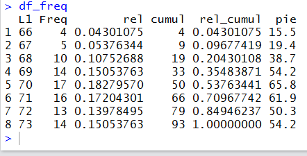
However, performing that command opens a new window in the upper left
corner of our RStudio session, and it places a nice table
view of df_freq in that pane. Figure 15 shows that table view.
Figure 15
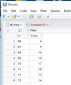
This is an even better view of the values that we want.
A small aside.
The work in preparation for this web page was done in a RStudio
session. The View(df_freq) command in just a straight forward R
session behaves in a slightly different fashion. In that
case, the View(df_freq) command opens a new window with the
values in it. A display of such a window is given in Figure 15a.
Figure 15a
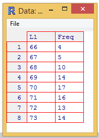
This window is not nearly as powerful as is the window in RStudio.
[We will see some of that power later on this page.]
However, it does look nice.
|
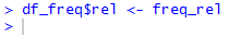
We want to add the values stored in freq_rel
to our data frame called df_freq.
We can do this by using the command
df_freq$rel<-freq_rel
This will create a new column in df_freq, called rel,
and assign the values found in freq_rel to that new column.
Please note that although we kept the names pretty similar,
there is no requirement to do so.
Figure 16 shows the command from the
Console pane in our RStudio
session.
Figure 16
After performing the command as shown in Figure 16,
we can look again at the Environment
pane in our RStudio session.
A portion of that pane is shown in Figure 17.
Figure 17
We can see, in Figure 17, that df_freq is
now a structure of 3 variables.
Looking back at the top left pane of the session,
shown in Figure 18, we see that without even asking for a redisplay,
the nice looking table
that we had created before has been augmented to show the new third column.
[Note that this automatic updating of the View result is another
difference between doing this in RStudio
versus doing it in straight R.
In straight R we would have to perform
another View(df_freq) command.]
Furthermore, the title of that column is now rel,
the name we used when we created it.
Figure 18
We continue the process by adding the other three columns with
the commands
df_freq$cumul<-freq_cumul
df_freq$rel_cumul<-freq_rel_cumul
df_freq$pie<-freq_pie
as shown in Figure 19.
Figure 19
And now, in our RStudio session,
the View display is updated to appear as in Figure 20.
Figure 20
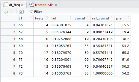
Back in the Console pane, if we just give the variable name, df_freq,
R displays, as shown in Figure 21, all of the values right there.
While not \as pretty as the other display, this may be adequate
for your needs. One advantage of this display is that you can
highlight and copy it so that you can paste it into another document,
possibly as input to some other program.
Figure 21
If all you want to do is to compute and display the
values that we have
found for our frequency table, then
there is no need to read further on this page.
All of the required steps are presented above and you can simply follow
those same steps for your next problem.
On the other hand, there is much more to see, both
in terms of the View() output in RStudio and
in terms of the codifying the numerous
steps that we took to generate the data frame.
The discussion below starts with two figures that illustrate some of the extra power
in the RStudio version of the View() display.
Following that there is a sequence of figures and the related text
to walk through a process to save and then re-use the steps that we went
through in creating the data frame.
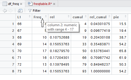
Taking a close look at Figure 20, you might notice that there is
something at the right end of each header cell in the table.
Figure 21a repeats that header row and circles, in red, that
special area in each header cell.
Figure 21a

If you point to the header cell, as shown in Figure 22, a small
box opens to give you information about that column.
Figure 22
If you are pointed at the header cell and click on it then
RStudio sorts the entire data frame on the basis of that column.
In Figure 22 we were pointing at the header cell for the Freq
column. We click on that header cell and the image becomes that of Figure 23.
Figure 23
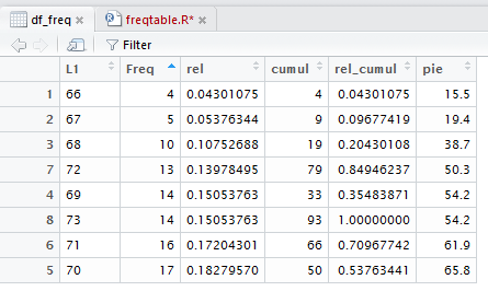
Notice in Figure 23 that the items in the Freq column are now in ascending
order.
Furthermore, the rest of the cells in the table have been rearranged so that the individual
rows of the table in Figure 23
are identical to the rows in Figure 22; the rows are just in a different order.
In fact, the first column which gives the position of the
"rows" of data in the original data frame still gives us that same information.
Thus, the value 72 which had been the 7th value in Figure 22,
is now the fourth value in Figure 23. However, 72 is matched with a Freq
value of 13 in both figures and Figure 23 still
tells us, via that first column, that 72 was the seventh item in the original structure.
Clicking on that same header cell again will reverse the sort as seen in
Figure 23a.
Figure 23a
As you might expect, particularly in a course such
as this one, there are many times when you might be asked to
create a frequency table from some data.
The process outlined in the various images above
is not too complex and not too long, but it is still a
pain to both remember and to perform.
It would be nice if we had a way to record that process and, essentially,
play it back when we need it. One way to do this is to create our own
function and to put the process into that function.
The rest of this page walks us through doing just that.
We really could create the new function in any text editor, but
since we already have an RStudio session open, we will do it right in this
session.
First, we need to create a new workspace.
We start by pointing to and then clicking on the File menu option.
This opens the option window on the left of Figure 24, the
window starting with New File. Then we point to that New File
option and just the action of pointing at it opens the secondary window to its right,
the one starting with R Script.
That is the option we want. Therefore, click on that
R Script selection. Figure 24 shows us pointing to that option.
Figure 24

That is the option we want. Therefore, click on that
R Script selection.
Clicking on that option opens a new workspace in the
upper left pane of the RStudio window. The blank, new workspace
is shown in Figure 25.
Figure 25
You might notice that the new workspace starts with the name Untitled1.
That will change later when we finally save the workspace as a file.
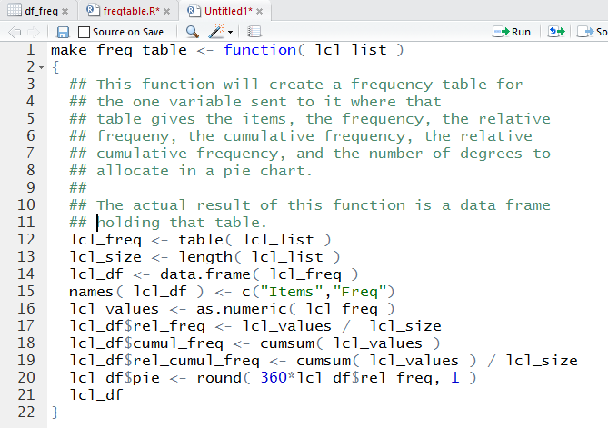
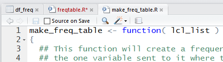
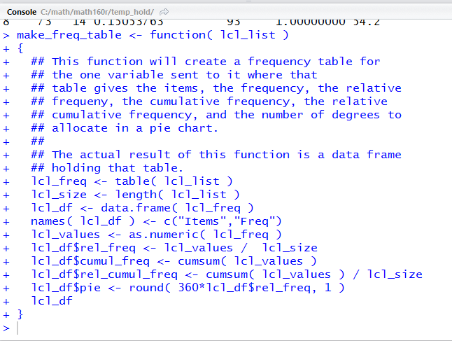
The function that we will create will follow the steps
that we took at the start of this page, although there are points where
two actions have been combined into one.
The function
is given by the following
lines of code:
 make_freq_table <- function( lcl_list )
{
  ## This function will create a frequency table for
  ## the one variable sent to it where that
  ## table gives the items, the frequency, the relative
  ## frequeny, the cumulative frequency, the relative
  ## cumulative frequency, and the number of degrees to
  ## allocate in a pie chart.
  ##
  ## The actual result of this function is a data frame
  ## holding that table.
  lcl_freq <- table( lcl_list )
  lcl_size <- length( lcl_list )
  lcl_df <- data.frame( lcl_freq )
  names( lcl_df ) <- c("Items","Freq")
  lcl_values <- as.numeric( lcl_freq )
  lcl_df$rel_freq <- lcl_values /  lcl_size
  lcl_df$cumul_freq <- cumsum( lcl_values )
  lcl_df$rel_cumul_freq <- cumsum( lcl_values ) / lcl_size
  lcl_df$pie <- round( 360*lcl_df$rel_freq, 1 )
  lcl_df
}
The lines are provided above so that you can, if desired, just copy them from this web page
and paste them into your new, blank workspace.
Alternatively, you could just type them into the workspace.
Discussing the meaning of the lines follows
Figure 26 because in that image of the lines we have line numbers provided by the RStudio
editor.
Figure 26
Here is a discussion of the lines in the workspace:
-
make_freq_table <- function( lcl_list )Assigns to the name make_freq_table a function
that will be defined by the rest of this line and all the rest of the lines
those enclosed by the { and } pair of characters.
Furthermore,
this function will have a single argument which we will call
lcl_list for the duration of the function definition. Our intent
is to be able to call this function and send to it a list of values.
Most likely that list will be in the variable L1 but it could
be in any variable. If the values are in L1 then we will call the function by
using the command make_freq_list(L1) in shich case lcl_list will be
assigned a copy of L1.
{ The squiggly brace on line 2 marks the start of the body of the function definition.
It will have to be matched by a closing squiggly brace at the end of the definition.
- As soon as we encounter a "pound sign", the # character,
the rest of the line is just a comment. It does nothing other than to explain to a human
reader what is going on here.
- More of the comment, but note that it is a matter of style to start with the double
##, a single one is sufficient.
- More of the comment.
- More of the comment, but note that even incorrectly spelled words may appear in a comment.
- More of the comment.
- More of the comment.
- More of the comment, though in this case it is just a blank comment used to put some spacing
into our overall comment.
- More of the comment.
- More of the comment.
lcl_freq <- table( lcl_list )
Use the table() function to
get a count of the differrent values that are
stored in lcl_list. Put that result in
lcl_freq.
lcl_size <- length( lcl_list )
Use the length() function to determine the
number of values in the lcl_list. Put that result in lcl_size,
lcl_df <- data.frame( lcl_freq )
Use the data.frame()
function to convert the 'table' that we created
in lcl_freq into a data frame.
names( lcl_df ) <- c("Items","Freq")
This is a command that we did not use originally,
but it was included here to force
the names of the two columns in lcl_df to
be Items and Freq, respectively.
lcl_values <- as.numeric( lcl_freq )
Use the function as.numeric()
to pull out the values that make up
the table that we had created.
We do this because it will make the next statement more clear.
lcl_df$rel_freq <- lcl_values / lcl_size
Compute the relative frequency by dividing the
frequency values by the number
of values in the original list.
Store this group of values in a new column of
lcl_df called rel_freq.
lcl_df$cumul_freq <- cumsum( lcl_values )
Use the
cumsum() function to get the cumulative sums and store those in
a new column of
lcl_df called cumul_freq.
lcl_df$rel_cumul_freq <- cumsum( lcl_values ) / lcl_size
Use the cumsum() function to find the cumulative
sum of values (this is a bit wasteful
since we had made this computation before,
but it jsut a wasted bit of machine time) and then divide those values by
the number of values in the original list.
Then store the results in
a new column of
lcl_df called rel_cumul_freq.
lcl_df$pie <- round( 360*lcl_df$rel_freq, 1 )
Compute 360 times the relative frequency values,
round the answers t 1 decimal place, and store the
results in
a new column of
lcl_df called pie.
lcl_df
Make the value of the function be the data frame
that we have created. This is important
in that if, later, we just call the
function make_freq_table() then the
result will be the data frame and R will display the
values in that data_frame.
However, if we call the function
make_freq_table() and assign it to a variabe,
then that variable will be assigned the value of the
data frame that we created in the function.
} Finally, the closing brace marking the end of our function definition.
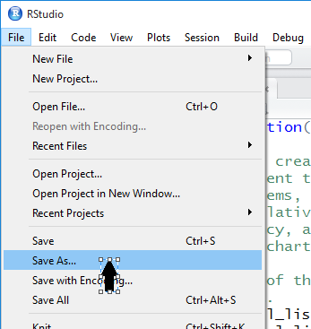
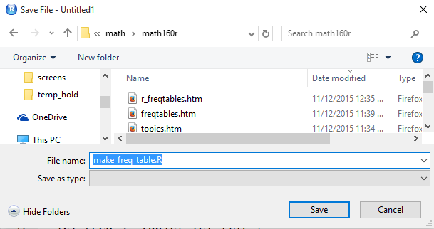
Having entered the code lines into the workspace,
our next task is to save this workspace as a file on the
computer. To do this we click on the File menu option.
RStudio opens the window shown in Figure 27.
Then we move the cursor down to the Save As... option.
Figure 27
When we click on the Save As... option, we get a new window, an
example of which is shown in Figure 28,
to help us name the new file and to locate that file
in whatever directory we desire. Assuming that the window shown in
Figure 28 has correctly identified the desired directory, note that we have given
the system a file name, in this case make_freq_table.R.
It is helpful, but not at all required, to have the name of the file be similar to
if not identical to the name of the function.
To actually save the file we click on the Save button.
Figure 28
Once the file has been saved, we note that the tab for the workspace
has changed from Untitled to make_freq_table.R as shown in
Figure 29.
Figure 29
It is important to note that at this point we have created and saved the file, but we have not told R
anything about the function we have designed.
There are two ways to tell R about this.
The first, illustrated here, is to highlight the entire
file (Alt-A is a good way to do this), and then
point to and click on the Run option at the top of the editor window.
Figure 30 shows everything highlighted and the cursor pointing to
the Run option.
Figure 30

When we click on that Run option RStudio submits
the highlighted lines to R in the Console window.
Figure 31 shows that submission in our Console window.
Figure 31
Once the function has been submitted, it is available for use.
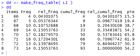
The commands
dd<-make_freq_table( L1 )
dd
cause R to run our newly defined function make_freq_table()
using L1 to give values to lcl_list in the function.
The result of the computations within the function,
namely the data frame constructed within the function,
is then assigned to the variable dd. The second line, dd
causes R to display the values now in dd.
All of this is shown in Figure 32.
Figure 32
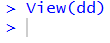
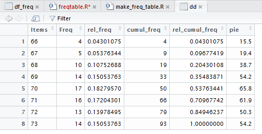
Then we give the command View(dd) as shown in Figure 33.
Figure 33
This creates a new tab in the top left pane
of our RStudio session, as shown in Figure 34.
Figure 34
In order to demonstrate a different method for loading the function
into R, we first close this session. That is shown in Figure 35.
Figure 35

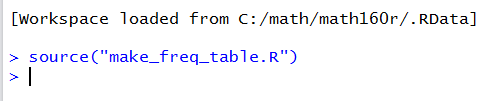
We will start from the beginning.
In Figure 36 we have started a new RStudio session,
which, in turn,
started a new R session in the Console window.
Then, because in our earlier session
we saved the entire function in a file called
make_freq_table.R,
we can use the command
source("make_freq_table.R")
to tell R to read the contents of that file
as if we had typed them into
our R session. This is done in Figure 36.
Note that the command here tells R
to load the function from the current working directory. This works because we saved
that function to this directory earlier. If we had wanted to load the function
from the parent directory which contains the functions I have provided,
then we would use the command
source("../make_freq_table.R") instead.
|
Figure 36
Note that there is no error or warning message as a resut of
our source() command. Furthermore, unlike our example in Figures 30
and 31, we did not have to highlight the code for the function
and the code of the function does not show up in
the Console area.
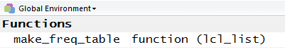
We can verify that make_freq_table() is again defined as a function
by looking in the Environment window.
There we will find make_freq_table identified as a current function.
We see this in Figure 37.
Figure 37
Because we are assuming this is a new session, we need to load
the gnrnd4() function, and then run it again.
This time we will
generate a different table of values, those in Table 5.
We construct the full, vertical
frequency table for the values in Table 5:
To make the same table in R we will use the following code lines
source("make_freq_table.R")
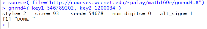
source( file="http://courses.wccnet.edu/~palay/math160r/gnrnd4.R")
gnrnd4( key1=546789202, key2=1200034 )
L1
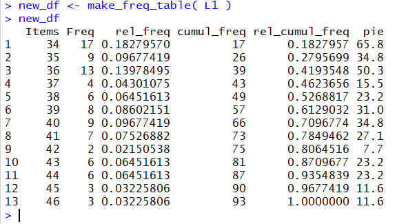
new_df <- make_freq_table( L1 )
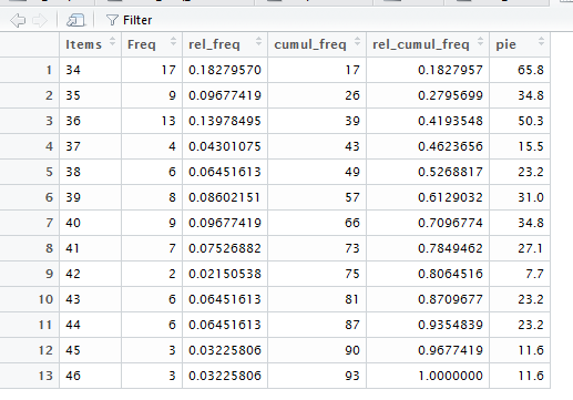
new_df
View( new_df )
to load the required functions, generate the data,
run the make_freq_table( L1 ) function
and store the result in new_df, display the contents of new_df
in the Console area, and finally via the view(nnew_df )
command, open a new window in our RStudio
session to display the table.
The first code line, source("make_freq_table.R") was discussed above.
Figure 38 show executing the second and third lines of code in the
Cpnsole window.
Figure 38
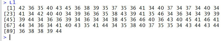
The fourth line of code, L1, just displays the
data values that we have generated. This is shown in Figure 39
and we can verify those values against the values in Table 5.
Figure 39
The next two lines of code,
new_df <- make_freq_table( L1 )
new_df
just call our function, passing the values in L1 to
that function, assign the result of the function to the variable new_df,
and finally display the contents of that new variable.
This is shown in Figure 40.
Figure 40
Finally, we use the code View( new_df ).
There is no result of this in the Console window, as seen in Figure 41.
Figure 41
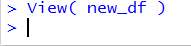
However, there is now a new display window giving the
table in a very nice form, as in Figure 42.
Figure 42
Here are lines of a script that, for the most part, duplicate the
lines of R used on this web page. Please note that where the script diverges
from the commands used above there are significant notes in the script
to guide you to appreciate and understand the changes.
# Frequency tables in R
#
#  For this script, rather than look for our files
#  in our "parent" folder, we will load them from
#  Palay's website.

source( file="http://courses.wccnet.edu/~palay/math160r/gnrnd4.R")
# generate the list of value shown on the web page
gnrnd4( key1=859459203, key2=800065 )
L1  #verify that we have the right values

# now try to use the built-in tabulate() function
tabulate(L1)
# That gave us more than we want

# shift over to use the built-in  table()  function
table( L1 )

# That gives us just the values that we want.
# However, let us store those values in a new variable
freq <- table( L1 )
freq  # and then look at what we have stored

# We notice that our variable  freq  holds both
# the names of the items and the values of the
# frequencies.  Let us pull those out, separately,
# and store them in their own variables

freq_vals<-as.vector(freq)
freq_names<-names(freq)
#  then look at what we have stored
freq_vals
freq_names

#  now we wwant to move on to finding the relative
#  frequencies.  To do that we need to divide each
#  frequency by the total number of items.

#  first get the total number of items
freq_size <- length(L1)
#  then compute the relative frequencies and save
#    those computed values in a new variable
freq_rel <- freq_vals/freq_size
#  now look at those values
freq_rel

#  Now we are ready to find the cumulative frequencies.
#  To do this we can use the built-in function cumsum().
#  And, we will store those values before we look
#     at them.
freq_cumul <- cumsum( freq_vals )
freq_cumul

#  Now it is an easy step to generate and then
#  look at the relative cumulative frequencies.
#  We just divide the cumulative frequencies by
#  the number of items, which we computed and
#  saved earlier.

freq_rel_cumul <- freq_cumul/freq_size
freq_rel_cumul

#  And, even though we know it is a bad idea to
#  make and use a pie chart, and even though R
#  would do that for us, it is a easy step to
#  compute the number of degrees to allocate
#  in a pie chart for each of the different
#  values in our data.  We just multiply the
#  relative frequencies by 360.  In this case we
#  take a further step and round that to one
#  decimal place.
freq_pie <- round(360*freq_rel,1)
freq_pie

#  So far we have computed all of the values that
#  we would include in a frequency table.  What we
#  have not done is to put all of those values
#  into a construct that will display the
#  completed frequency table in R.

#  We will do that now but putting copies of
#  the desired variables into a dataframe.

df_freq <- data.frame( freq)
df_freq

#  With that simple start we have the beginning
#  of our "vertical" frequency table.

# We will take a small step sideways here to
#  look at another way that R can display that
#  table.  We can use the View() function to
#  do that.  Be sure to note the capital V.
View(df_freq)

# Now we can return to our task of building
# our complete frequency table.  We can add the
# relative frequencies to our dataframe
df_freq$rel <- freq_rel

#  and we could get a new view of that dataframe
View(df_freq)

# Now complete our build by adding the other
#  three columns.
df_freq$cumul <- freq_cumul
df_freq$rel_cumul <- freq_rel_cumul
df_freq$pie <- freq_pie

# again, we can use View() to see this table
View(df_freq)

# or we could go back to our old method and
#  just look at it in the console display
df_freq

# the web page on this topic goes through the step
# to create a new function that captures
# all of the steps that we have taken to
# make a frequency table.

# Here we will just load that function, again this
# time from Palay's web page rather than from
# the parent directory.
source( file="http://courses.wccnet.edu/~palay/math160r/make_freq_table.R")

# now that the function make_freq_table() is loaded
# into our environment we can use it to duplicate
# all of the painful work that we did above in lines
# 21 through 108.

dd <- make_freq_table( L1)
dd

# Or we could use View() to get the nicer
# looking table.
View( dd )

# The we page goes on, building on the fact that
# there were instructions on the web page for
# actually creating and saving the function in
# our current directory, to show an alternative
# way to load the function.  We did not create
# that local version of the function, but we
# do have a version in our parent folder.  So,
# we will demonstrate here how to load functions
# from our parent folder.

#  First, we will use the dangerous but effective
#  command rm() to wipe out our entire environment.
rm( list=ls() )

#  Notice the environment is now empty.
#  First we want to use gnrnd4() to generate some
#  values.  To do this we need to load gnrnd4()
#  into our environment.

source("../gnrnd4.R")
# now generate the values in Table 5 of the
# web page.
gnrnd4( key1=546789202, key2=1200034 )
L1 # just to verify the values

# now we want a full frequency table for those
# values.  We can use make_freq_table() to do
# this, but first we need to load the function.
source("../make_freq_table.R")
new_df <- make_freq_table( L1 )
new_df
View( new_df )

# Having seen this, with just a few commands we
# now have a way to generate full frequency
# tables.

# in fact, given that we have make_freq_table()
# in our environment, we can generate a large
# data set and then apply our function to that
# to get a new frequency table.
source("../gnrnd5.R")
gnrnd5(78034095603, 13000045)
head( L1,20)
tail(L1, 20)
make_freq_table( L1 )
Return to Topics page
©Roger M. Palay
Saline, MI 48176 November, 2015