Probability: Discrete Cases

Return to Topics page
Fortunately, the general introduction to probability page used discrete cases for all of its examples. In discrete cases the random variable can only have values that are from a hopefully small set of distinct values. Thus, flipping a coin results in "head" or "tails". Rolling a die results in a value 1, 2, 3, 4, 5, or 6. Choosing a single candy from a container of M&M's might result in a candy that is one of a few colors (possibly Red, Green, Blue, Orange, Yellow, or Brown). These are all discrete cases and, from the long discussions in the introductory page, we know how to assign and use probabilities for these kinds of situations.

As a quick review, consider the case shown in Table 1.

Expected Value

In order to talk about expected value we will consider the random variable defined by Table 2.

Table 2
Values	3	4	7	9	14	15	20	24
Frequency	2	2	2	4	3	2	1	1
Probability	2/17	2/17	2/17	4/17	3/17	2/17	1/17	1/17

If X is the random variable defined by Table 2, then the expected value of X is denoted as E(X). The meaning of the expected value is "If we take repeated samples, each of size 1, with replacement, from the distribution of values defined by Table 2, and we looked at the mean of all those samples, what is the anticipated value of that mean?" It certainly isn't the mean of the different values. We need to take the frequency of the different values into account.

Because we know the frequency of each value, we really could expand the table into the population 3, 3, 4, 4, 7, 7, 9, 9, 9, 9, 14, 14, 14, 15, 15, 20, 24. Of course, the mean of that population, which is the sum of all the values divided by the number of values, is exactly the anticipated value if we were to find the mean of repeated samples of size 1 taken with replacement from that population.

In order to facilitate the following discussion, we will rename some of the values that we are using. The original "values" in Table 2 we will refer to as v_i so v₅=14. The original "frequencies" in Table 2 we will refer to as f_i so f₅=3. The expanded population of values that we created we will refer to as y_i so y₅=7 and y₁₆=20. We know that the expected value of the y's, E(Y), is equal to the expected value of the v's, E(V).

We could express the computation as

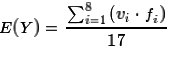
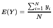Then too, thinking about how we got the "sum of the y_i's, we could have found the same total by looking at the sum of the product of the values and their respective frequencies,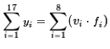

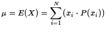
. That means that we could rewrite the equation for expected value as

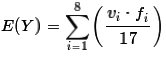
. However, mathematically, because the denominator is a constant in the problem, we can move the denominator into the summation to rewrite it as

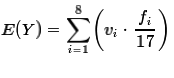
. Then, rearranging the factors inside the summation we get

. But the factor

is just the associated probability

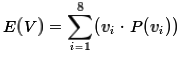
. Making that change and remembering that E(V)=E(Y) produces the form that we often see for the expected value, namely,

.

Of course, for the more general case where we have N different values (x₁, x₂, x₃, ... x_N-1,x_N) each with a frequency (f₁, f₂, f₃, ... f_N-1,f_N) so that the probability of each is given by P(x_i)=f_i/N we would write this as

Let us see how we can do this computation in R. Figure 1 shows the commands that we could use to recreate the data in Table 2.

Figure 1

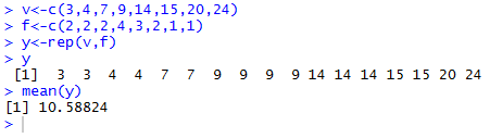
The command v<-c(3,4,7,9,14,15,20,24) creates the data values in v. The command f<-c(2,2,2,4,3,2,1,1) creates the frequencies in f. The next command, r<-rep(x,y), uses the replicate function rep(). That function creates the long list of the different values, each repeated the number of times indicated by the corresponding frequency held in f. The long list is stored in y. We can see that long list by just giving R the variable name y. As we see, in Figure 1, that list is exactly the list that we created by hand above. Our goal was to find the mean of that expanded list of values. We can do that in R by using the command mean(y). The console image in Figure 1 shows that the mean, and thus the expected value, is 10.58824.

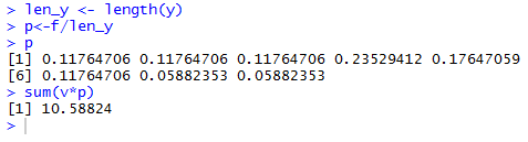
The other approach to finding the expected value was to use the formula

. We need to create those probabilities. Each probability is just the frequency divided by the number of items in the population. There are many ways to get the number of items, len_y<-length(y) being one of them. Then the code p<-f/len_y creates the probabilities and assigns them to p. Therefore, we can have R perform this alternate computation of the expected value by using the command sum(v*p). This is shown in Figure 2.

Figure 2

And, as expected, we get the same answer.

To illustrate a use for the expected value we will talk about playing a game. Actually, there are two versions of the game.

Version 1	Version 2
We have a game piece with 17 faces. The faces are marked with 3, 3, 4, 4, 7, 7, 9, 9, 9, 9, 14, 14, 14, 15, 15, 20, and 24, respectively. Each face is equally likely to "come up" when we roll the piece.	We have a game piece with 8 faces. The faces are marked 3, 4, 7, 9, 14, 15, 20, and 24, respectively. The game piece is "weighted" so that there is not an equal likelihood of "coming up" for each face. In fact, P(X=3)=2/17, P(X=4)=2/17, P(X=7)=2/17, P(X=9)=4/17, P(X=14)=3/17, P(X=15)=2/17, P(X=20)=1/17, and P(X=24)=1/17.,

With that design it does not make any difference which version of the game we are playing. In either version we roll the game piece and look at the value on the face that "comes up". Were we to play each version over and over and record the values that "come up" we could not distinguish between the recordings. The values, the 3, 4, 7, 9, 14, 15, 20, and 24, have the same probability of showing up in either version of the game.

Now let us make this a bit more "interesting". We will change the game into a form of gambling. You pay for the opportunity to play the game, to roll the game piece. After the roll I will pay you the number of dollars indicated by the face that "comes up". Thus, if you roll a 20 then I will pay you $20. If you roll a 7 then I will pay you $7. Oh, and by the way, I am charging you $12 to play the game, that is, $12 each time you roll the piece.

To some this might look like a good deal. After all, the most you can lose is $9 on a roll (if you roll a 3) and you could win upwards of $8 or $12 if you roll a 20 or a 24. However, because we have learned about expected value, and because we have done the calculations above, we see that the expected value of this game is $10.59. That means that if we play the game long enough our average "winning" will be really close to (using the Law of Large Numbers) $10.59. But is costs us $12 to play each time. Or, in other words, our average loss will be $1.41 for each roll of the piece. The game favors me, the "house", because although you might play and even start out winning if I can keep you playing then, over time, I am going to come out way ahead. In fact, I will average winning $1.41 for each time that you play.

Should you ever play this game? That depends upon your financial limitations, your time limitations, and, most importantly, if you can get me to play the game where you only have to pay $10 for each roll. If you have the time and money to last through a possible "string of bad luck", that is, getting a lot of low numbers for a while, and if you can get me to only charge you $10 for each roll, then playing is a good idea. On average you will win $0.59 a roll. If you can play this game for 1000 rolls you should, at the end of the 1000 rolls, be "up" by around $590. Almost certainly you will not be "up" by exactly that amount, but you should be close to that. How "close"? Well, that is a topic that we will discuss below, but for this particular game, "close" is going to mean that we will almost certainly be ahead, maybe by only $100 or maybe by $1100, but most likely we will be ahead by somewhere in between those values, usually closer to the $590 value.

We will try that. I have created that exact game in this web page and we will now roll the piece 1000 times. Here is the record of our results (we play this anew each time we refresh the page): (I trust you will forgive me for not printing out the 20,000 game results.)

Variance and Standard Deviation of Discrete Distributions

Just before we ran the 1000 games reported above, there was a statement that although we expect to be "up" by about $580 the most we can say is that our winnings should be "close" to that value. Then we said that for this distribution and for 1000 games, "close' means that our winnings will most likely be between $100 and $1100 but centered around the $590 value. If you did as was requested and reloaded the page, a number of times, at that point then you should have seen the idea of "close" play out as predicted. I know that when I have done this to see twenty pages, I have seen winnings as low as $357 and as high as $873. Interestingly, the mean of those 20 values was $601.65, not far at all from the $589 that was predicted.

We know that one measure of dispersion for our distribution is the standard deviation. And we recall that the symbol for the standard deviation is σ. Also, σ² is the variance. Furthermore, if we have a population of N items called y_i then the standard deviation is given by

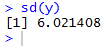
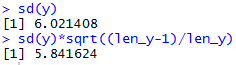
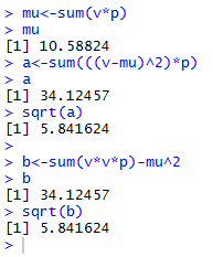
. But, back in Figure 1, we actually created our y_i's. Therefore, we might assume that we can get the standard deviation of our distribution by giving the command sd(y). This does give us a value, as shown in Figure 3, but we have forgotten one thing.

Figure 3

We got an answer, but we need to remember that the R function sd() computes the standard deviation of a sample not the standard deviation of a population. Our random variable distribution is a population. We need to make an adjustment to the original computation done by sd(). As we have seen in an earlier page, the adjustment is to multiply that answer by the square root of the quotient of (N-1) and N, where N is the number of items in the population. That computation is shown in Figure 4.

Figure 4

Figure 4 shows us that the standard deviation of our discrete random variable, defined by Table 2, is 5.841624.

Just as a small reminder, we did develop a small function called pop_sd() to find the population standard deviation. The code for that function was:

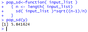
pop_sd<-function( input_list )
  { n <- length( input_list)
    sd( input_list )*sqrt((n-1)/n)
  }

If we have defined that function in our current session, then we could get the result by using the command pop_sd(y). All of this is shown in Figure 5.

Figure 5

It is always nice to get the same answer!

What we just did was to find the standard deviation of the discrete distribution by creating the equivalent long list of values that we called y_i and then computing the standard deviation of that population. We would like to be able to compute the same value directly from the values in Table 2, without having to create the expanded list of values. To do this we can use the formula

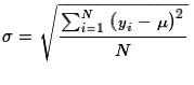
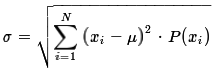
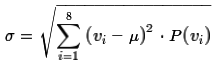or the formula

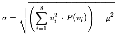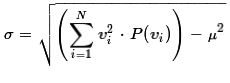
. If we were doing the computation by hand the latter formula is easier to use. As we see in Figure 6 we can easily use either formula in R.

Figure 6

In summary, for the more general case where we have N different values (x₁, x₂, x₃, ... x_N-1,x_N) each with a frequency (f₁, f₂, f₃, ... f_N-1,f_N) so that the probability of each is given by P(x_i)=f_i/N we would write this as

And, of course, the variance, σ², is just the square of the standard deviation, σ.

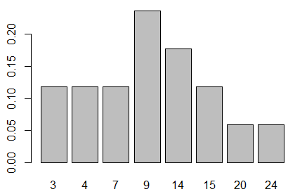
Before we leave this topic it is worth looking at a few bar charts of the probability distribution. The first attempt at this is to use just the simple command barplot(p,names.arg=v). The result is shown in Figure 7.

Figure 7

The vertical values displayed in Figure 7 are the probability values that we saw as decimal values back in Figure 2. We can "pretty-up" the graph by adding a few directions to the barplot() command. Using

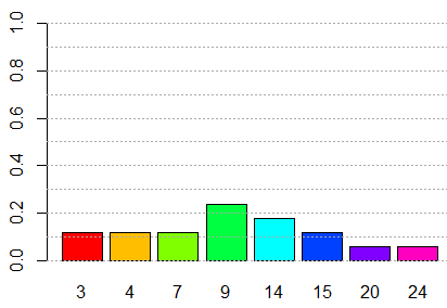
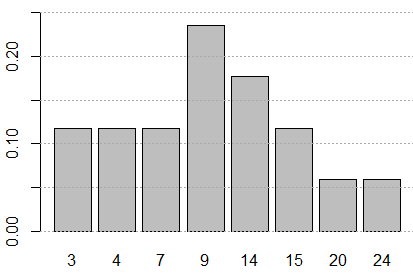
barplot(p,names.arg=v, ylim=c(0,.25))
abline(h=seq(0,.25,.05),col="darkgray", lty=3)

produces Figure 8.

Figure 8

The bars in Figure 8 represent the various probabilities. All the bars are the same width, so the magnitude of the probability being represented is shown both by the height of the bar and by the area of the bar. In that same sense, we could say that the probability of getting a random variable from this distribution such that the value of the random variable is strictly less than 14 is represented by the total area of the bars to the left of 14.

A little more work, using

barplot(p,names.arg=v, ylim=c(0,1), col=rainbow(8))
abline(h=seq(0,1,.1),col="darkgray", lty=3)

yields Figure 9. The vertical scale in Figure 9 was extended to run from 0 to 1, in part so that we can see that if we were to "stack up" all the bars, the total stack would be the full height of the plot. This should not be a shock since we know that the sum of all the probabilities must be 1.

Figure 9

Then, just to reinforce the relationship between "frequencies" and "probabilities", Figure 10 shows a bar chart based on the frequencies that we are using. The image is essentially identical to that of Figure 7.

Figure 10