Probability: Chi-Squared Distribution

Probability: χ² Distribution

Introduction
The χ² Distribution: Graphs and Tables
pchisq() in R
qchisq() in R
Sample Problems
Listing of all R commands used on this page

Introduction

The third to last letter in the Greek alphabet is χ (lower case) Χ (upper case). It is given the name chi and it is pronounced with a hard ch as we use it in chronic and a long i as we use it in idol. Thus, chi sounds as sky without the initial s.

We use the letter χ to help us name yet another probability distribution. This is the χ² distribution, also written as the chi-squared distribution. We will use both versions of the name in part because when we finally get to the R functions for this distribution they will use the chisq name.

We have already seen the standard normal distribution and the Student's t distribution. In both cases these were symmetric with the line of symmetry being x=0. We used this symmetry to great advantage as we looked at the areas in the tails of the distributions.

We did see that the Student's t distribution had different forms depending upon the number of degrees of freedom specified. The lower the number of degrees of freedom the flatter is the Student's t distribution. That is, the lower the number of degrees of freedom the more area we find under the curve further away from 0. This is a major flattening for low values of the degrees of freedom but by the time we get to 5 degrees of freedom there is less than 2% of the area further away from 0 (in both tails) than the t-score 3.37. By the time we get to 10 degrees of freedom there is less than 2% of the area further away from 0 than the t-score 2.77.

There were two consequences of all of this. First, for the standard normal and Student's t we could create tables of the cumulative probability distribution and keep the x and t scores in the range of -3.7 to 3.7. (There were even pointers to tables that used the symmetry aspect to cut this down to values from 0 to 3.7.) Second, for the Student's t we saw that rather than have 50 or 100 of those tables, one for each different degree of freedom, we could just have one table with the critical values of t for just some special areas in the tail of the distribution for different degrees of freedom. Thus, we looked at such popular values as 0.0005, 0.001, 0.0025, 0.005, 001, 0.05, and 0.10 or the area in the tail. That convenience allowed publishers to just use one page for the Student's t table instead of having a whole section of the book for multiple tables. Of course, all that goes out the window once we can just compute values for the distribution on the calculator or computer.

The χ² Distribution

The χ² distribution also changes for different degrees of freedom. However, the χ² distribution is not symmetric and it is defined only for positive values. A few illustrations should help here.

Graph 1	Graph 2	Graph 3
Graph 4	Graph 5	Graph 6

The shape of the χ²distribution changes dramatically across these graphs. We can see that the graph is only defined for positive x values. We can see that the graph is not symmetric. We can see that as the number of degrees of freedom increases most the area under the graph moves to the right and it flattens out.

We could set things up so that we have a cumulative probability table for each different number of degrees of freedom. Here is a link to a page that asks you for the number of degrees of freedom and then allows you to generate such a cumulative probability table. Try this for a several different degrees of freedom. The tables are quite different and quite long. It should not come as a shock to find that we do not want to have a table of cumulative probabilities for each different number of degrees of freedom. Rather, most statistics books give us a table of "convenient" critical values for the χ² distribution. One web page of such values is at The Chi-Squared Critical Values Table.

Figure 1 shows the top of that table.
Figure 1

We could use that table to say for 1 degree of freedom an x-value 3.841 has 0.05 as the area under the curve and to the right of 3.841. Still with 1 degree of freedom the area under the curve and to the right of 5.024 is 0.025 square units. What we cannot read from the table, but the value is consistent with the values in the table, is that the area under the curve and to the right of x = 4.00 is approximately 0.04550026 square units.

For 2 degrees of freedom the area under the curve and to the right of 4.605 is 0.010 square units. That is, for a χ² distribution with 2 degrees of freedom the probability that we get a value of 4.605 or greater is 0.010. Again, what we cannot see from the table is that for a χ² distribution with 2 degrees of freedom we have P( x > 4 ) ≈ 0.1353353. The modified graphs below show and give the area under the curve for various degrees of freedom for x-values > 4.

Graph 7 P(x > 4) ≈ 0.04550026	Graph 8 P(x > 4) ≈ 0.1353353	Graph 9 P(x > 4) ≈ 0.4060058
Graph 10 P(x > 4) ≈ 0.8571235	Graph 11 P(x > 4) ≈ 0.9989033	Graph 12 P(x > 4) ≈ 1

We do need to note here that although the area reported in Graph 12 is given as 1 that is just the true value expressed to 7 significant digits and then rounded off. In other words, the true value is not 1, but there is so little area under the curve and to the left of 4 that when we round off the value of the area to the right of 4 the answer rounds to 1.0000000.

Returning, for a moment, to the table of values, we note that the choices for the convenient areas, the column headings, seem a little strange. Later when we are really using the χ² distribution, we will want to find values such as "What is the critical value for 7 degrees of freedom that has 1% probability of getting that value or less than that value." The table only gives the right tail! Therefore, we would look in the table to find the value for 7 degrees of freedom that has a probability of 99% of getting that value or more than value. In the table we would find that value to be 1.239. That becomes P(x < 1.239) = 0.01.

Before leaving the graphs and tables, we should at least combine the graphs 1 through 6 into one graph. This is the way that most books present the graphs of the χ² distribution. That unified graph is shown in Figure 2.

Figure 2

pchisq() in R

As we have seen in other distributions, the use of tables is now essentially obsolete. In R we have a function, namely pchisq() that compute the area under the χ² curve for a specific number of degrees of freedom and either to the left or to the right of a specified value. The commands

# look at areas to the right of 4 for 6 different
# options on the degrees of freedom
pchisq(4,1, lower.tail=FALSE)
pchisq(4,2, lower.tail=FALSE)
pchisq(4,4, lower.tail=FALSE)
pchisq(4,8, lower.tail=FALSE)
pchisq(4,16, lower.tail=FALSE)
pchisq(4,32, lower.tail=FALSE)

were used to find the areas reported above in graphs 7 through 12. The console view of those commands is shown in Figure 3.

Figure 3

The syntax of the pchisq() command is displayed in the hint, shown in Figure 4, that R gives us when we start typing the command.

Figure 4

We need to specify a value, shown as q, and the degrees of freedom, shown as df. If we say nothing more, then R will assume that we want the lower tail area, that is, the left tail area. [This is a functionality that we do not get directly from the table.] As we saw in Figure 3, if we want the upper tail area then we need to include the directive lower.tail=FALSE. This use of the lower.tail direction is consistent with the other probability commands that we learned earlier for the normal and Student's t distributions.

Then too, the one left tail value that we saw above was P(x < 1.239) = 0.01. We had to do some creative reading from the table to get that. However, the R command pchisq(1.239,7) should give us the value in just one simple statement. This is shown in Figure 5.

Figure 5

The actual computed result while different from 0.01 is a more accurate approximation. We will see later that the x-value that we want to use in order to have 0.01 as the area to the left of that value, with 7 degrees of freedom is slightly different from 1.239. The 1.239 and the 0.01 came from the tabular values above and represent significant rounding.

qchisq() in R

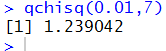
The qchisq() function in R allows us to specify a desired area in a tail and the number of degrees of freedom. From that information, qchisq() computes the required x-value to get the specified area in the specified tail with the specified number of degrees of freedom. Thus, the command qchisq(0.01,7) asks R to find the x-value that has 0.01 area to its left, with 7 degrees of freedom. The result is shown in Figure 6.

Figure 6

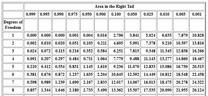
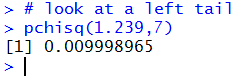
Recall that the table value had been 1.239 to produce P(x < 1.239) = 0.01, but that our earlier use of the command pchisq(1.239,7) had shown that this was not quite accurate. Now we see that using the value 1.239042 should produce better results. We can test that with the command pchisq(1.239042,7) to get the result shown in Figure 7.

Figure 7

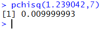
We did not hit the target 0.01 but we are a lot closer than before. All of this should remind us that we are always dealing in approximations for these values. Without infinite precision we will never get infinitely accurate results. However, the good news is that we rarely need anything like the extra precision shown here. The table view kept us at 3 decimal places, and that is usually quite enough. The default R view holds 7 significant digits and that will always be enough, though we have seen that we can get even more digits displayed in R by changing the option that controls the number of digits in the display.

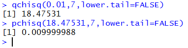
We should take note that by a simple change in the command to qchisq(0.01,7,lower.tail=FALSE) we get the x-value such that 1% of the area is to the right of that value, again for 7 degrees f freedom. The console record of that command and the confirming pchisq(18.47531,7,lower.tail=FALSE) command is in Figure 8.

Figure 8

Sample Problems

We will solve the eight problems:

For a χ² distribution with 6 degrees of freedom, what is the probability of having a random event X be less than 2.34?
For a χ² distribution with 9 degrees of freedom, what is the probability of having a random event X be greater than 15.34?
For a χ² distribution with 17 degrees of freedom, what is the probability of having a random event X be less than 6.66 or greater than 27.34?
For a χ² distribution with 14 degrees of freedom, what is the probability of having a random event X be between 5.25 and 25.41?
For a χ² distribution with 5 degrees of freedom, what is the x-score that has 0.0333 square units under the curve and to the left of that x-score?
For a χ² distribution with 25 degrees of freedom, what is the x-score that has 0.125 square units under the curve and to the right of that x-score?
For a χ² distribution with 11 degrees of freedom, what are the x-scores that hav 0.75 square units under the curve and between those x-scores with the tails having equal areas?
For a χ² distribution with 23 degrees of freedom, what are the x-scores that have 0.0333 square units under the curve and to the outside the interval between those x-scores where the tails have equal areas?

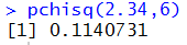
1. The first problem becomes P(X < 2.34) for 6 degrees of freedom. The R statement to get this value, pchisq(2.34,6), and the answer are shown in Figure 9.

Figure 9

2. The second problem becomes P(X > 15.34) for 9 degrees of freedom. The R statement to get this value, pchisq(15.34, 9, lower.tail=FALSE), and the answer are shown in Figure 10.

Figure 10

3. The third problem becomes P(X < 6.66 or X > 27.34) for 17 degrees of freedom. The R statement to get this value, pchisq(6.66, 17) + pchisq(27.34, 17, lower.tail=FALSE), and the answer are shown in Figure 11.

Figure 11

4. The fourth problem becomes P( 5.25 < X < 25.41) for 14 degrees of freedom. The R statement to get this value, pchisq(25.41, 14) - pchisq(5.25, 14), and the answer are shown in Figure 12.

Figure 12

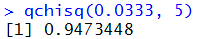
5. The fifth problem becomes find a value for x such that P(X < x) = 0.0333 for 5 degrees of freedom. The R statement to get this value, qchisq(0.0333, 5), and the answer are shown in Figure 13.

Figure 13

6. The sixth problem becomes find a value for x such that P(X > x) = 0.125 for 25 degrees of freedom. The R statement to get this value, qchisq(0.125, 25, lower.tail=FALSE), and the answer are shown in Figure 14.

Figure 14

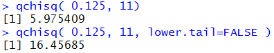
7. The seventh problem becomes find a value for x₁ and x₂ such that P(x₁ < X < x₂)= 0.75 for 11 degrees of freedom. Stated that way there is no unique solution. However, the problem statement included the stipulation that the area in the two tails needed to be equal. But if the area between the two values is 0.75 then the total tail area must be 0.25 square units. Thus, the area to the left of x₁ must be 0.125 square units and the area to the right of x₂ must be 0.125 square units. This means that we have P( X < x₁ ) = 0.125 and P( X > x₂ ) = 0.125. The R statements to get these values are qchisq( 0.125, 11) and qchisq( 0.125, 11, lower.tail=FALSE ). Those statements and the answers are shown in Figure 15.

Figure 15

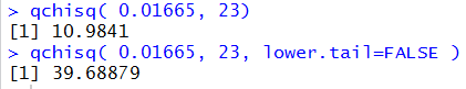
8. The eighth problem becomes find values for x₁ and x₂ such that P(X < x₁) + P(X > x₂)= 0.0333 for 23 degrees of freedom. Stated that way there is no unique solution. However, the problem statement included the stipulation that the area in the two tails needed to be equal. Thus, the area to the left of x₁ must be 0.01665 square units and the area to the right of x₂ must be 0.01665 square units. This means that we have P( X < x₁ ) = 0.01665 and P( X > x₂ ) = 0.01665. The R statements to get these values are qchisq( 0.01665, 23) and qchisq( 0.01665, 23, lower.tail=FALSE ). Those statements and the answers are shown in Figure 16.

Figure 16

Listing of all R commands used on this page

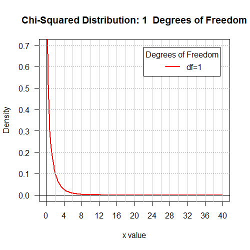
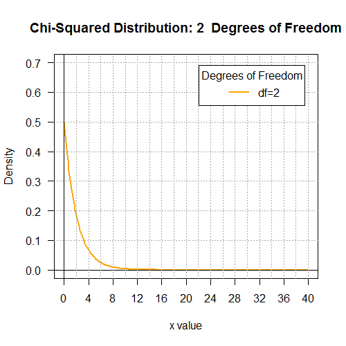
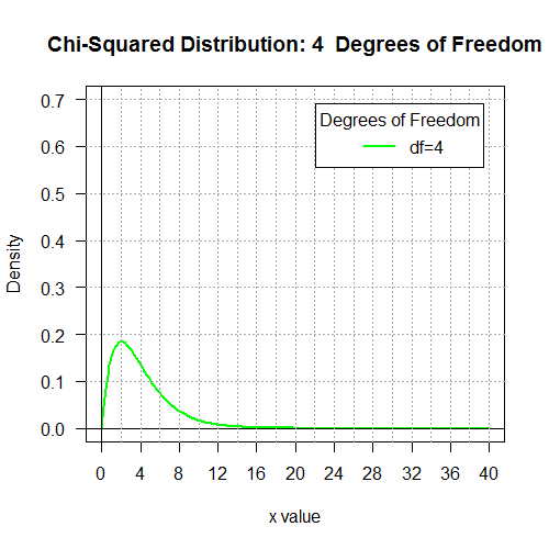
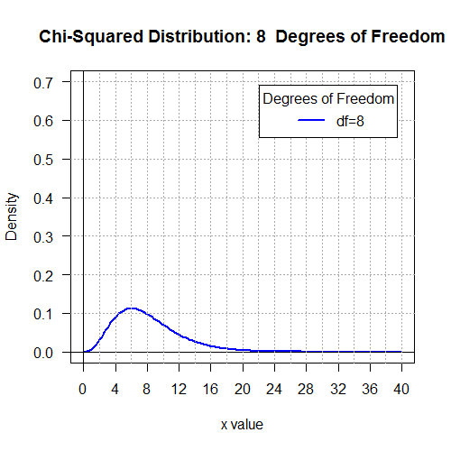
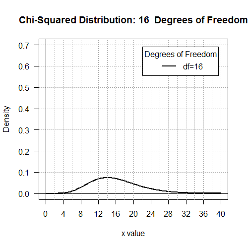
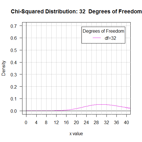
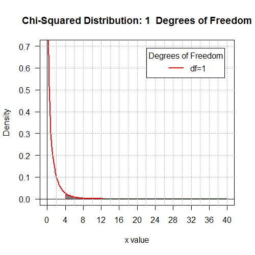
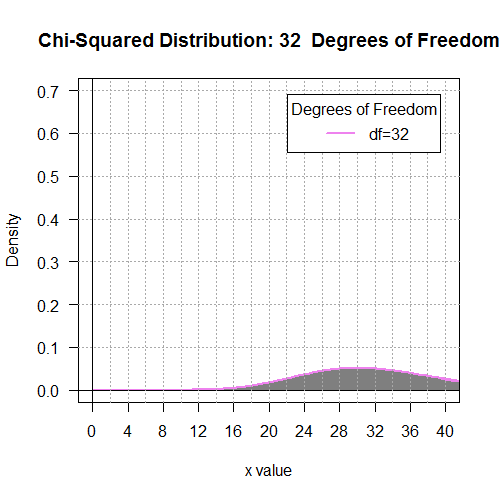
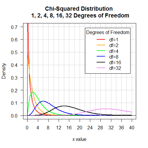
# Display the Chi-squared distributions with
#  1, 2, 4, 8, 16, and 32 degrees of freedom. 

x <- seq(0, 40, length=200)
hx <- rep(0,200)

degf <- c(1,2,4,8,16,32)
colors <-  c("red",  "orange", "green", "blue", "black", "violet")
labels <- c("df=1",  "df=2",  "df=4",  "df=8",  "df=16",  "df=32")

plot(x, hx, type="n", lty=2, lwd=2, xlab="x value",
     ylab="Density", ylim=c(0,0.7), xlim=c(0,40), las=1,
     xaxp=c(0,40,10),
     main="Chi-Squared Distribution \n 1, 2, 4, 8, 16, 32 Degrees of Freedom"
     )

for (i in 1:6){
  lines(x, dchisq(x,degf[i]), lwd=2, col=colors[i], lty=1)
}
abline(h=0)
abline(h=seq(0.1,0.7,0.1), lty=3, col="darkgray")
abline(v=0)
abline(v=seq(2,40,2), lty=3, col="darkgray")
legend("topright", inset=.05, title="Degrees of Freedom",
       labels, lwd=2, lty=1, col=colors)


for (j in 1:6 ){
plot(x, hx, type="n", lty=2, lwd=2, xlab="x value",
     ylab="Density", ylim=c(0,0.7), xlim=c(0,40), las=1,
     xaxp=c(0,40,10),
     main=paste("Chi-Squared Distribution:",k[j]," Degrees of Freedom")
     )

for (i in j:j){
  lines(x, dchisq(x,degf[i]), lwd=2, col=colors[i], lty=1)
}
abline(h=0)
abline(h=seq(0.1,0.7,0.1), lty=3, col="darkgray")
abline(v=0)
abline(v=seq(2,40,2), lty=3, col="darkgray")
legend("topright", inset=.05, title="Degrees of Freedom",
       labels[j], lwd=2, lty=1, col=colors[j])
  
}

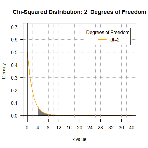
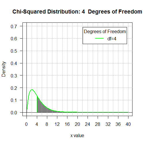
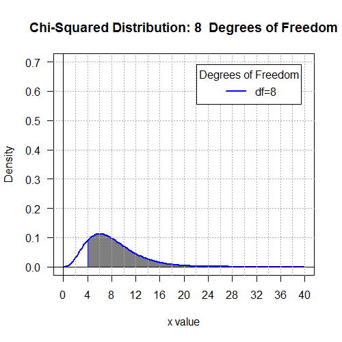
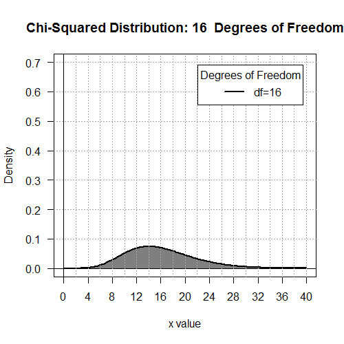
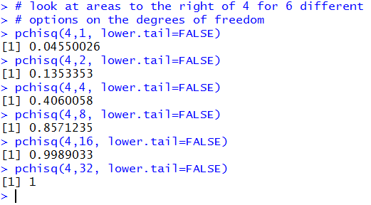
# look at areas to the right of 4 for 6 different 
# options on the degrees of freedom
pchisq(4,1, lower.tail=FALSE)
pchisq(4,2, lower.tail=FALSE)
pchisq(4,4, lower.tail=FALSE)
pchisq(4,8, lower.tail=FALSE)
pchisq(4,16, lower.tail=FALSE)
pchisq(4,32, lower.tail=FALSE)

# look at a left tail
pchisq(1.239,7)

qchisq(0.01,7)
pchisq(1.239042,7)

qchisq(0.01,7,lower.tail=FALSE)
pchisq(18.47531,7,lower.tail=FALSE)

pchisq(2.34,6)
pchisq(15.34, 9, lower.tail=FALSE)
pchisq(6.66, 17) + pchisq(27.34, 17, lower.tail=FALSE)
pchisq(25.41, 14) - pchisq(5.25, 14)
qchisq(0.0333, 5)
qchisq(0.125, 25, lower.tail=FALSE)
qchisq( 0.125, 11)
qchisq( 0.125, 11, lower.tail=FALSE )
qchisq( 0.01665, 23)
qchisq( 0.01665, 23, lower.tail=FALSE )