Probability: Binomial Distribution

Return to Topics page

The Binomial distribution refers to a whole class of discrete distributions. The Binomial distribution occurs in cases where
  1. We have a fixed number of trials (i.e., attempts) are done (run n trials).
  2. There are only 2 possible outcomes of each trial: one is called a success, the other called a failure.
  3. The probability of success is the same for each trial. We designate the probability of success on any one trial as p. This means that the probability of a failure is (1-p).
  4. The trials are independent; knowing the outcome of one trial tells you nothing about the outcome of the next trial.
  5. We are looking at a random variable, X, that is the number of successes in those n trials.
For example, if we start with a coin that has a 56% probability of coming up heads when we spin the coin. We will spin it 5 times (there are 5 trials). On each spin the probability of getting heads is 0.56. The spins are independent events; the coin does not change its behavior based on its history of spins. We want to know the probability that we will get each of the following: 5 heads, 4heads and 1 tail, 3 heads and 2 tails, 2 heads and 3 tails, 1 head and 4 tails, and 5 tails. This situation where we have n=5 and p=0.56, is one instance of a binomial distribution. If we change the value of n and/or we change the value of p we get a different instance of a binomial distribution.

We could use a tree diagram to compute the various probabilities. Alternatively, we can just look at the six possible results (getting 5, 4, 3, 2, 1, or 0 heads). The probability of getting 5 heads is just p5. The probability of getting 5 tails is just (1-p)5 The probability of getting the sequence HHHHT is just p4(1-p). However, this is but one of five ways to get 4 heads and 1 tail, namely, HHHHT, HHHTH, HHTHH, HTHHH, and THHHH. Each will have the same probability. Therefore, the probability of getting 4 heads and 1 tail is 5p4(1-p). In that expression, the 5 represented the number of combinations of 5 things taken 4 at a time. We recall that we represent that as 5C4. Using that we could write our probability as 5C4p4(1-p)1.
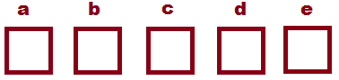
Why do we look at this as combinations? Really, we have five spots to fill, one for each spin of the coin. If we call the spots a, b, c, d, and e, then the question becomes which of the five slots get the 4 heads?
There are 5 combinations of the five slots taken 4 at a time, namely, abcd, abce, abde, acde, and bcde. If for each of those combinations you place a head (H) in the named slot, and then fill the one empty slot with a tail (T), then you will get the five choices given above, in order. We will do this again for the next situation.
One way to get 3 heads and 2 tails is HHHTT. The probability of getting that sequence is p3(1-p)2. However, HHHTT is but one of the 10 combinations of 5 things taken 3 at a time, namely, HHHTT, HHTHT, HHTTH, HTHHT, HTHTH, HTTHH, THHHT, THHTH, THTHH, and TTHHH.
Again, we have five spots to fill, one for each spin of the coin. If we call the spots a, b, c, d, and e, then the question becomes which of the five slots get the 3 heads?
There are 10 combinations of the five slots taken 3 at a time, namely, abc, abd, abe, acd, ace, ade, bcd, bce, bde, and cde. If for each of those combinations you place a head (H) in the named slot, and then fill the two empty slots with a tail (T), then you will get the ten choices given above, in order.
With 10 different ways to get 3 heads and 2 tails the probability of getting that result is 10p3(1-p)2 or, using the combinations format, 5C2p3(1-p)2.

We can see the pattern develop. For 5 trials, our probability of getting k successes, which we should write as P(X=k) but which we often write as P(k), is given by
P(X=k) = 5Ckpk(1-p)5-k
In fact, could make this even more general and say for n trials the probability of getting k successes, which we should write as P(X=k) but which we often write as P(k), is given by
P(X=k) = nCkpk(1-p)n-k
For p=0.4 and n=5 we get the following probabilities:
This little list of values is nice to have, but it is but one instance of a binomial distribution. It gives the value for the particular case where n=5 and p=0.40. What about other cases, where is some other value and/or p is some other probability.

For years people have created tables that give binomial probabilities for lots of different values of n and many "common" values of p. I have a web version of tables like this at Binomial Distribution Tables. A portion of the table for n=5 is given in Figure 1 with the column for p=0.40 highlighted.

Figure 1

The values in the highlighted column of the table are just the values that we listed above. But the rest of that table gives the binomial distribution values for other values of p that are multiples of 0.05. Other tables on the web page provide the same kind of information for different values of n, the number of trials.

What are we supposed to do if we are using the tables and we want n=5 but p=0.37? If all we have are the tables we could do the basic computations ourselves, or we could interpolate between values in the table. Thus, when n=5, p=0.37, we use the table shown in Figure 1 and note that the P(X = 3) will be between P(X = 3) for p=0.35 and P(X = 3) for p=0.40, that is between 0.1811 and 0.2304. The difference between those values is 0.2304 - 0.1811 = 0.0493. Our desired p value is 0.37 and that is 2/5 of the way between 0.35 and 0.40. Therefore, we want to go 2/5 of the 0.0493 along the way from 0.1811 toward 0.2304. But 2/5 of 0.0493 is 0.01972 and 0.1811+0.01972 = 0.20082 which we would round off to 0.2008 because we should not be adding any significant digits. Thus, using the table our best guess is that for p=0.37 we have P(X = 3)=0.2008. (As we will see below, a more accurate answer is 0.2010418, but our interpolated value of 0.2008 is not that far off from there.)

Although it is nice to be able to find P(X = k) in the tables for a given n and p, we often want to know things like P(X ≤ k). For example, staying with our case of n=5 and p=0.40, to find P(X ≤ 3) we would just add the values in the cells of the table for P(X = 0), P(X = 1), P(X = 2), and P(X = 3). To help in this we mimic the list above to produce
The web page Binomial Distribution (Cumulative) Tables has tables arranged using this scheme. A portion of the table for n=5 is given in Figure 2, again with the column for p=0.40 highlighted.

Figure 2

Before leaving these tables, we should note that we could reconstruct values in Figure 1 from those in Figure 2. For example, still with n=5 and p=0.40, P(X = 3) = P(X ≤ 3) - P(X ≤ 2), or, from the table in Figure 2, P(X = 3) = 0.9130 - 0.6826 = 0.2304, the value that we had in Figure 1.

Using the web, and the programming that we can put into web pages, it is now possible to create a different table for binomial probabilities. Starting at Set Up Binomial Table we can produce specialized tables for any desired number of trials and any specified probability of success.

The printed version of either of the first two web pages discussed above would require 13 sheets of paper. Even with that we only get tables for the values of n from 2 to 30, and only the columns of values for p as the 19 multiples of 0.05. Prior to advanced hand-held calculators, doing the computations by hand was pretty much out of the question. Certainly a language such as R should give us some way to compute these values directly!

The pbinom(k,n,p) function in R computes P(X ≤ k) for n trials with p the probability of a success. Notice that this computes the probability of getting k or fewer successes in n trials, not the probability of getting exactly k successes. Therefore, the command 
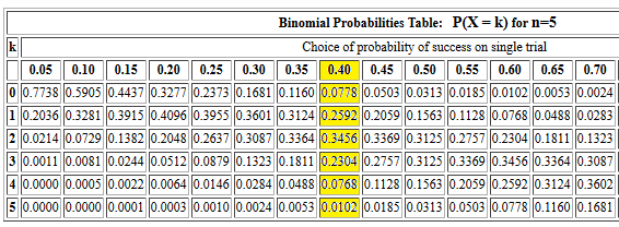
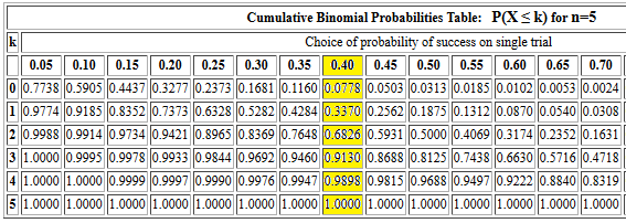
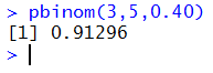
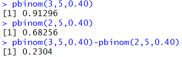
pbinom(3,5,0.40) should produce the same value that we found in Figure 2 for the cumulative probability of getting 3 or fewer successes out of 5 trials, each with a 0.40 probability of success. The console record of that command is given in Figure 3.

Figure 3

This value, when rounded to 4 places, is the same as we had in Figure 2.

If we want to find P(X = 3) using R then we will have to employ the equation P(X = 3) = P(X ≤ 3) - P(X ≤ 2). Figure 4 shows computing the two values, just so that we can confirm them, and then the difference in the values to get the desired P(X = 3).

Figure 4

That last value, 0.2304, corresponds to the same value in Figure 1.

With the pbinom() function we are not limited to the multiples of 0.05 for the values of the probability for success. We can get a direct answer for our earlier question of P(X = 3) for n=5 and p=0.37 by using the command 
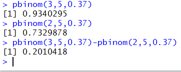
pbinom(3,5,0.37)-pbinom(2,5,0.37) as eventually shown in Figure 5.

Figure 5

That is the source of the "more correct" answer given above when we got an approximate answer from the table by interpolating values.

This business of having to do the subtraction to find the probability of getting an exact number of successes can be a bit tiring. Perhaps we should look at some way to just get the answer. We can do this by letting R do all of the work via a new function that we will build. The code for that function is:
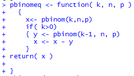
pbinomeq <- function( k, n, p )
  {
    x<- pbinom(k,n,p)
    if( k>0)
    { y <- pbinom(k-1, n, p)
      x <- x - y
    }
return( x )

}
The console image of defining the function is given in Figure 6.

Figure 6

And two examples of using the new function, using values that we already computed, are given in Figure 7.

Figure 7

As noted before, it is nice to get a confirmation of earlier work!

At this point we really have all that we need for computing binomial probabilities. However, there are many ways to ask the question. Consider the following. If the probability of success in a binomial distribution is 0.42 and we do 34 trials, what is the probability of getting
  1. less than or equal to 11 successes?
  2. less than 11 successes?
  3. exactly 11 successes?
  4. more than 11 successes?
  5. equal to or more than 11 successes?
  6. no fewer than 11 successes?
  7. no more than 11 successes?
  8. something other than 11 successes?
  9. between 11 and 18 successes, including 11 and 18?
  10. between 11 and 18 successes, excluding 11 and 18?
  11. less than 11 or more than 18 successes?
  12. less than or equal to 11 or more than or equal to 18 successes?
Let us go through each of those.
  1. less than or equal to 11 successes: This is the meaning of the standard call to the pbinom() function. Thus the command pbinom(11,34,0.42) will give us the answer 0.1672396.
  2. less than 11 successes: This is equivalent to finding the probability of getting 10 or fewer successes. Thus the command is pbinom(10,34,0.42). The answer is 0.09292053.
  3. exactly 11 successes: We can do this as the probability of getting 11 or less minus the probability of getting 10 or less. To do that we could use 
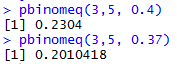
pbinom(11,34,0.42)-pbinom(10,34,0.42) t get the answer 0.07431911. Alternatively, if we have loaded our function pbinomeq() then we can use it as pbinomeq(11,34,0.42) to get the same 0.07431911.
  4. more than 11 successes: This is the complement of having 11 or fewer successes. Thus, we are really looking at 1-P(X≤11) which becomes 1-pbinom(11,34,0.42) which gives us 0.8327604. Alternatively, we could look at this as the probability of getting 12 or more successes. One might think that the command pbinom(12,34,0.42,lower.tail=FALSE) would compute this. However, the documentation for R states that for the pbinom() function lower.tail logical; if TRUE (default), probabilities are P[X≤x], otherwise, P[X>x]. Therefore, if we specify lower.tail=FALSE we will not be including the first value since we are then looking at a "greater than" situation. If we choose to use the lower.tail=FALSE option we need to start at a value below 12. Therefore the command we want is pbinom(11,34,0.42,lower.tail=FALSE) which yields the same result, 0.8327604.
  5. equal to or more than 11 successes: Now we can compute not getting 0 through 10 successes via 1-pbinom(10,34,0.42) to get 0.9070795, or we could use the lower.tail=FALSE approach , remembering to adjust the first argument to the function and use the command pbinom(10,34,0.42,lower.tail=FALSE) to get 0.9070795.
  6. no fewer than 11 successes? "No fewer than 11" means "11 or more". We did this before as 1-pbinom(10,34,0.42) or pbinom(10,34,0.42,lower.tail=FALSE) to get 0.9070795.
  7. no more than 11 successes: "No more than 11" means "11 or fewer" which we did as pbinom(11,34,0.42) which gave us 0.1672396.
  8. something other than 11 successes: This is the complement of having exactly 11 successes. We could play with the pbinom() function but it s easier to just use the pbinomeq() function as 1-pbinomeq(11,34,0.42) to get the answer 0.9256809.
  9. between 11 and 18 successes, including 11 and 18? Here we find the probability of getting 18 or fewer and then subtract the probability of getting less than 11. We can do this via the command pbinom(18,34,0.42)-pbinom(10,34,0.42) to get the result 0.8349292.
  10. between 11 and 18 successes, excluding 11 and 18: This is similar to the previous case except that we no longer want to include 18 and 11. We just need to adjust the command as pbinom(17,34,0.42)-pbinom(11,34,0.42) to get the result 0.7008324.
  11. less than 11 or more than 18 successes: This is just the complement of the probability of having between 11 and 18 successes (including the 11 and the 18) so we can code this as 1-(pbinom(18,34,0.42)-pbinom(10,34,0.42)) which gives the answer 0.1650708.
  12. less than or equal to 11 or more than or equal to 18 successes: This is just a slight change from the previous problem in that we now include 11 and 18 in the answer, not in the part being excluded. The command has to become 1-(pbinom(17,34,0.42)-pbinom(11,34,0.42)) which gives the answer 0.2991676.


Now we want to look at the mean, variance, and standard deviation of the binomial random variable. In doing this we need to point out that these are parameters of the distribution, not statistics drawn from a sample distribution. That is, if we have a binomial random variable X for the case where n=5 and p=0.40, then there is a mean for this, called μX, a variance, called σX2, and a standard deviation, called σX, for that distribution. If we have a sample from that distribution then we expect that the sample statistics will be close to, though not the same as, the distribution parameters.

Before we look at the parameter values let us look at a sample, or at many samples since the sample presented in Figure 8. There we have a display of 1500 experiments where each experiment involves 5 trials of a spin of a coin that is weighted so that it shows up as heads 40% of the time. For each experiment we record, and display in Figure 8 the number of successes, i.e., "heads", that we get in the 5 trials.

Figure 8: changes with each reload


Those values change with each reload of this web page because the data in Figure 8 represents 1500 experiments. However, we have equations that give us the mean, variance, and standard deviation for the ideal binary distribution with n=5 and p=0.40. Those equations are: You can reload this page many times and the statistics from the actual experiments should always be close to the parameters just given for the ideal distribution.

These distribution parameters will come in handy later, after we have learned of the normal distribution and in those cases where we are using a binomial distribution but one with more trials than we can handle with the tables and more trials than we can handle with the software. In those cases, these parameters can be used to get a normal approximation to the binomial distribution. At this point in the course these parameters just remain interesting values, although we do recall that the mean is the expected value.

Return to Topics page
©Roger M. Palay     Saline, MI 48176     December, 2015