The Power of a Test
Return to Topics page
The pattern that we have seen for formulating a
test of a null hypothesis starts with
-
stating the null hypothesis,
- stating an alternative hypothesis,
and
- setting a level of significance.
The null hypothesis is always stated as "the value of some
parameter of the population is equal to
some specific value.
For example, for the mean of a population we might have
-
H0: μ = 4
as the null hypothesis,
- H1: μ < 4
as the alternative hypothesis, and
- 0.05 as the level of significance.
It is because we have a specific value for the
parameter as given in the null hypothesis
that we can formulate the probability of getting
the associated sample statistic at certain values.
For example, if we have a population with a
normal distribution and with a known
standard deviation of 4, σ=4,
we might look at the null hypothesis that the mean of
the population is 4,
H0: μ = 4.
We know that for a sample of size 16
the distribution sample means, x,
from that population, assuming that H0
is true, will be N(μ,σ/sqrt(n)) which for this case will be
N(4,4/sqrt(16)) = N(4,1).
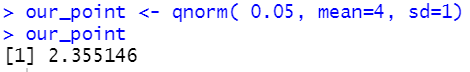
And, we can use
| Statements | Console output |
our_point <- qnorm( 0.05, mean=4, sd=1)
our_point
|
|
to determine that, for a sample of size 16, the probability of getting a sample mean
that is
2.355146
or lower is 5%. We visualize this as the area under the normal
curve for a N(4,1) distribution, to the left of
the value 2.355146 is 0.05.
We can see this in Figure 1.
Figure 1
Distribution of the sample mean.
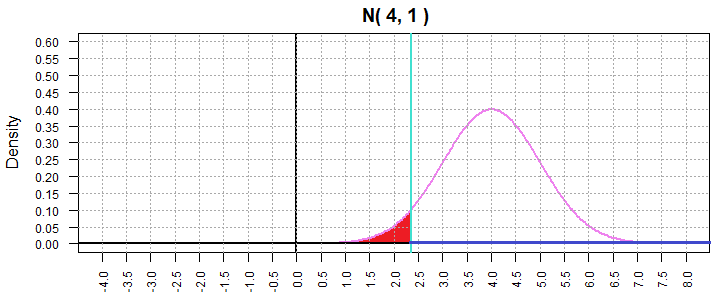
The shaded area in Figure 1 represents 5% of the
total area under the curve. [In fact, the total area under the curve
is 1 square unit and the shaded area is
0.05 square units.]
We have been using that kind of model to determine
the critical values and the attained significance
in
our hypothesis tests.
In a situation as shown in Figure 1,
we know that if the null hypothesis is true then, for a sample of size 16, the
probability of getting a sample statistic, the sample mean, that is
2.355146 or lower is 5%. For a one-sided test,
H1: μ < 4, we set that
value, 2.355146, as the critical value.
We say that we will
reject H0, at the 0.05
level of significance, if we get a sample mean
less than 2.355146.
Remember, it is entirely possible to get a sample statistic
of 2.355146 or lower even if the null hypothesis is true,
but getting such a value should only occur about 5% of
the time. That is, we are willing to make a Type I
error, rejecting the null hypothesis when it is in fact true,
5% of the time.
We captured this arrangement in a table similar to that
given below as Table 1.
| Table 1 |
| | The Truth (reality) |
| Our Action |
H0 is TRUE |
H0 is FALSE |
| Reject H0 |
This is a
Type I error |
made the
correct
decision |
Do not
Reject H0 |
made the
correct
decision |
This is a
Type II error |
We went on to say that we will
use the symbol α, the lower case Greek letter "alpha", for the probability of making a
Type I error, and that α
is the significance of the test.
Naturally, we want α to be small. We do not
like making errors!
The other type of error that we can make is a
Type II error, not rejecting H0
when it is in fact false. We use the symbol β, the lower case Greek letter "beta",
for the probability of making a Type II error.
Again, we do not want to make errors. However,
this kind of error is much harder to control
or even compute.
Consider the example shown in Figure 1.
There, for the distribution of the sample mean,
we have σ=1 and H0: μ = 4
and H1: μ < 4.
Our critical value became 2.355146. If we select a random sample of size 16
from the population and the sample mean is less than 2.355146 then we reject
H0 in favor of H1.
This leaves us with a 5% chance of
making a Type I error. But what is
the value of β, the probability of
not rejecting H0 when it is in fact
false.
We know that we will not reject H0
if we our sample mean is greater than 2.355146.
How likely is that? We cannot answer that by looking at
Figure 1 because Figure 1 shows the case where
H0 is true and β, the probability of making
a type II error, assumes that
H0 if false.
The challenge is that we have no idea just how far
"false" H0 will be.
For example, if μ = 1.9 then H0
is false. But the same is true if μ = 2.3, or if
μ = 0.9, or if
μ = 3.6, or if μ = any other value less than
4.
We will continue to examine this by looking at a few different cases.
First, look at the
case where the true value for μ
is really 1.9. Clearly, 1.9 is less than 4.
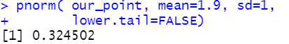
If that is true, then the chance of our choosing a value
greater than 2.355146 is easy to compute using
| Statements | Console output |
pnorm( our_point, mean=1.9, sd=1,
       lower.tail=FALSE)
|
|
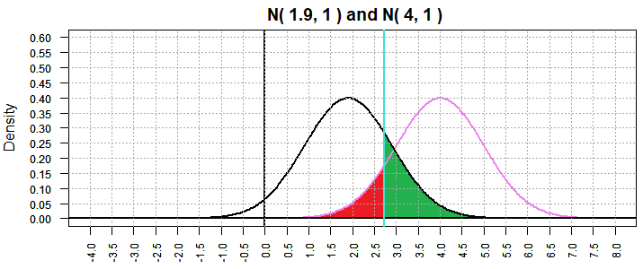
and that value is 0.324502.
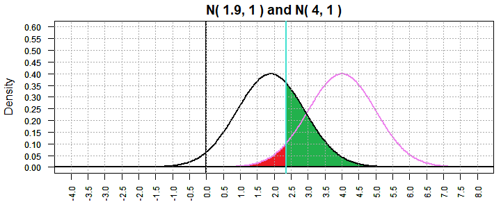
This is shown in Figure 2 where the "red" area is the probability
of making a type I error if H0: μ = 4 is true
and the "green" area is the probability of making a type II
error testing H0: μ = 4 when in fact
μ = 1.9.
Figure 2
Our first observation will be that for any particular situation if we decrease α then we will increase β.
For the situation above where we are testing
H0: μ = 4 against
H1: μ < 4. Now decrease α to be 0.02.
[Remember that we are looking at a normal population with known
σ=4 and we are taking samples of size 16. That makes the distribution of
sample means N(4,4/sqrt(16)).]
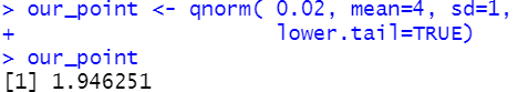
That change in α moves our "critical value" for the N(4,1)
distribution of the sample means down to 1.946251.
| Statements | Console output |
our_point <- qnorm( 0.02, mean=4, sd=1,
                    lower.tail=TRUE)
our_point
|
|
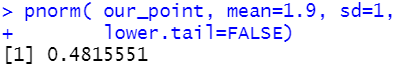
But, in the process of moving the critical value lower, we have
increased the area under the N(1.9,1) curve and to the right of the
critical value to 0.4815551.
| Statements | Console output |
pnorm( our_point, mean=1.9, sd=1,
       lower.tail=FALSE)
|
|
All of this is shown in Figure 3.
Figure 3
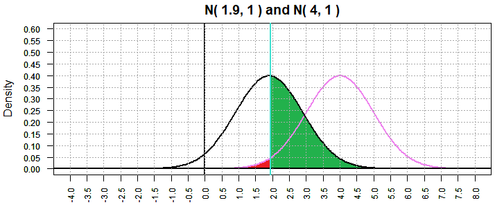
The "red" area is still α and the "green" area is still β.
As per the discussion above
we have α=0.02 and β=0.4815551. It would seem the
using a smaller α results in a larger β.
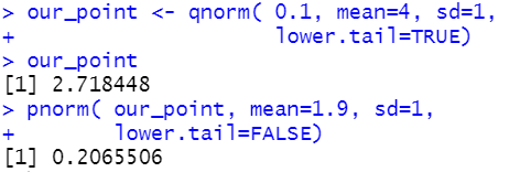
We can test this out by doing the problem again, but this
time with α=0.10. This makes the critical value 2.718448
and causes the value of β to drop to 0.2065506.
| Statements | Console output |
our_point <- qnorm( 0.1, mean=4, sd=1,
                    lower.tail=TRUE)
our_point
pnorm( our_point, mean=1.9, sd=1,
       lower.tail=FALSE)
|
|
The result is shown in Figure 4.
Figure 4
Again, this demonstrates that the lower we make α the higher
we force β.
Let us change our focus. Now we will look at the effect of changing our
choice for the alternative "false" value of μ.
The example shown in Figure 2 above considered the situation where
we were looking at the size of our type II error for a test of
H0: μ = 4 against
H1: μ < 4 and where the
true value of μ was 1.9.
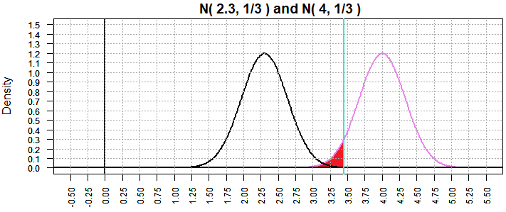
Now look at a similar situation, again with α=0.5, where we consider that
true value of μ is 2.3, just another of the infinitely many
options for the situation where H0 is not true.
Because we have returned to α=0.5 our graph of the N(4,1)
is unchanged and the critical value is again 2.355146, just as it was for Figure 2.
However, as shown in Figure 5, the graph of N(2.3,1) is a shift to the
right from Figure 2.
Figure 5
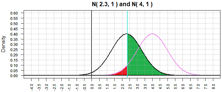
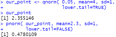
Therefore, the area that is shaded green, the representation of
the probability of making a type II error, has increased. We went from
0.324502 in Figure 2 to 0.4780109 in Figure 5. We can calculate
the latter from
| Statements | Console output |
our_point <- qnorm( 0.05, mean=4, sd=1,
                    lower.tail=TRUE)
our_point
pnorm( our_point, mean=2.3, sd=1,
       lower.tail=FALSE)
|
|
It appears that as we look at "true" values of μ that get closer to
our null hypothesis, 4, we see an increase in the probability of making
a type II error.
We can check this out by looking at another case, this time where the
"true" value that we are using to compute β is further away from
our null hypothesis value. In particular, Figure 6 shows the
situation where the "true" value is
0.9.
Figure 6
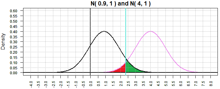
Now the probability of making a type II error has dropped to
0.07281437. This seems to confirm our observation.
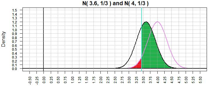
We can get a further confirmation by setting the "true" value even closer to
our hypothesis value of 4. Figure 7 looks at the case where the
"true" value is 3.6.
Figure 7
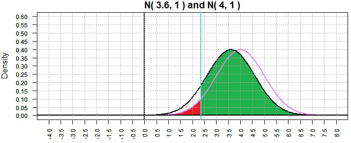
That is an enormous probability of making a type II error;
β=0.8934072.
So far we have seen two things that can change the probability of making a
type II error:
- Making α smaller results in increasing β
- Making our choice of the "true" value of μ closer to
the hypothesis value of μ increases β
There is a third factor that has an effect of changing β,
namely, increasing the sample size. All of the work done above was had a sample size of 16.
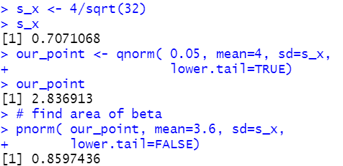
What happens if we have a sample size of 32? Now the sample mean will
have a distribution with
a standard deviation equal to 4/sqrt(32) which simplifies to 1/sqrt(2).
We will revisit the case shown in
Figure 7 but this time with the standard deviation set to 1/sqrt(2).
This is shown in Figure 8.
Figure 8
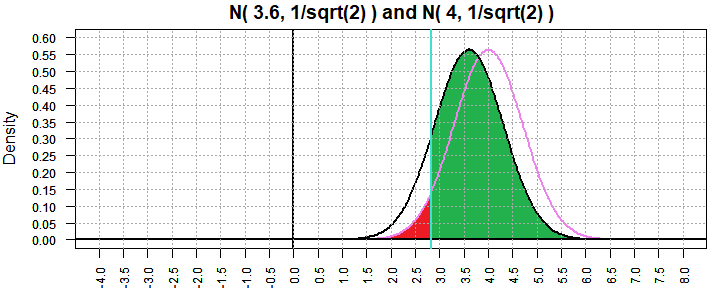
The plot of the two distributions has changed, the "bell" is narrower and taller, although the center of
each "bell" is unmoved. The critical value is now 2.836913 and there is still
5% of the area to its left. The green region representing β is
still large, but it has gone down from 0.8934072 to 0.8597436.
| Statements | Console output |
s_x <- 4/sqrt(32)
s_x
our_point <- qnorm( 0.05, mean=4, sd=s_x,
                    lower.tail=TRUE)
our_point
# find area of beta
pnorm( our_point, mean=3.6, sd=s_x,
       lower.tail=FALSE)
|
|
Let us check the other cases to see
if increasing the sample size reduces the probability of making a type II error.
Back in Figure 5 we considered the "true" mean to be 2.3 and the result
was β=0.4780109. Now, with sample size 32, and thus a standard deviation
of the sample means equal to
of 1/sqrt(2), we have Figure 9 where β is now 0.2238337.
Figure 9
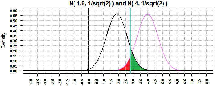
In Figure 2 we considered the "true" mean to be 1.9 and the result
was β=0.324502. Now, with sample size 32, and thus a standard deviation
of the mean in samples is
1/sqrt(2), we have Figure 10 where β is now 0.09258643.
Figure 10
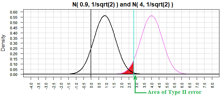
In Figure 6 we considered the "true" mean to be 0.9 and the result
was β=0.07281437. Now, with sample size 32, and thus a standard deviation
of sample means
of 1/sqrt(2), we have Figure 11 where β is now 0.003079366.
Figure 11
We will take this further by increasing the sample size to 144, making the
standard deviation of the sample means have the value 4/sqrt(144)=1/3.
[This will make each "bell" more narrow and taller. Note the change in both the
vertical and horizontal scales in the figures below.]
Returning to the case in Figure 11 where the "true" mean is 0.9, we now get
Figure 12 where β has dropped to 9.654609e-15.
Figure 12
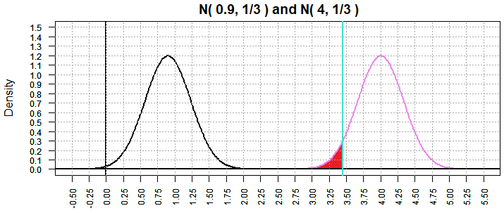
[A note should be made here to point out that the horizontal and vertical
scales have changed. As the standard deviation drops, more of the area under
each curve is closer to the mean of the curve, thus driving up the vertical scale.
This also brings the tails of the curves closer to the mean. Had the
horizontal scale remained as above then most of the width of the
graph would be empty space. Changing the horizontal scale allows us to focus on the
portion of interest.]
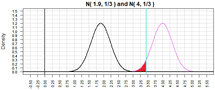
Returning to the case in Figure 10 where the "true" mean is 1.9, we now get
Figure 13 where β has dropped to 1.618753e-06.
Figure 13
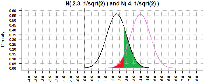
Returning to the case in Figure 9 where the "true" mean is 2.3, we now get
Figure 14 where β has dropped to 0.0002749971.
Figure 14
Returning to the case in Figure 8 where the "true" mean is 3.6, we now get
Figure 15 where β has dropped to 0.6717872.
Figure 15
The pattern has been consistent across all of these examples. Increasing the
sample size drives down the standard deviation of the sample mean and as
a result this drives down the associated value of β, the probability
of making a type II error.
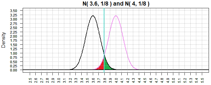
Still, in Figure 15, we had a considerable value for β, namely,
0.6717872. Following our pattern, if we increase the sample size again, we
should be able to lower that probability. Figure 16 shows the result of
increasing the sample size to 1024, making the standard deviation of the
sample mean be 4/sqrt(1024), or 1/8. Indeed, this brought the value of β down to
0.05995561. [Again, note that the scales changed for Figure 16.]
Figure 16
We can now restate the list of things that affect our level of β:
- Making α smaller results in increasing β
- Making our choice of the "true" value of μ closer to
the hypothesis value of μ increases β
- Increasing the sample size results in decreasing β.
The Power of a test
All of the discussion above has focused on β, the probability of making
a type II error. However, the common practice is to talk about the power of a test
which is 1-β. Naturally, as β gets smaller, the power of the test
gets larger.
The issue that has been demonstrated above but that has not been resolved is the
question of selecting a "true" value for the population parameter so that we can
measure β and thus find the power of the test. Clearly, we
can manipulate the power of a test simply by changing the assumed alternative
"true" value of the population parameter.
In a statistics course it is almost always the case that if you are asked to compute
the power of a test then you will be given the value to use in that computation.
But being given the alternative does not help us select an appropriate
alternative in the real world.
In practice, it is probably best to choose a "true" value
that represents the point where the
result of the original test
will make a difference in what you (or someone else) is doing.
For example, let us say that the situation above
represents the drift of some instrument. By "drift" we mean that although the instrument
is supposed to produce a specific value in some setting, the instrument really
produces a value near the expected value. For example, I have a Keurig coffee machine.
If I press one of the buttons then the machine is supposed to pump out 8 ounces of hot water.
Now, in reality it never does this exactly, but it is close, never over 8 ounces, but often less
to one extent or another.
I am sure that the Keurig company is aware of this "inaccuracy".
They might want to run a test on their machines looking at the
null hypothesis H0: μ = 8
against the alternative hypothesis
H1: μ < 8.
They could decide to do this test with a sample of machines and that they would
be happy with a test level of significance α=0.02. They
chose 0.02 because they decided that if the null hypothesis is rejected
as a result of the test then they may have to redesign and replace the mechanism that
measures the amount of water pumped through the system. This would be
an expensive change. With this small α it is unlikely
that they will reject H0 if it is true.
But, they also want a large power of the test, i.e., a small
β.
As we have seen, the Keurig company can decrease β by
increasing α (which they do not want to do), by increasing the
sample size (this could get expensive too), or by choosing a "true" value
that is far from the null hypothesis value, in this case, 8.
The decision on what alternative "true" value to use might come down to
market research saying "We know that customers start to get really ticked off
if, when they push the button for 8 ounces, they only get 7 or fewer ounces."
Therefore, Keurig sets the "alternative true value" at 7. Now they can
adjust the sample size to get the power of the test to be whatever
is their desired value, say 0.95, by setting the sample size so
that the value of β is driven down to 0.05.
One last word on the subject.
Remember, remember, remember, that the power of the
test depends upon the alternative "true" value that you are given
or the value that you choose for the alternative to the null hypothesis.
There should be some good reason why that value was chosen
and a good reason is not that it makes the test seem more powerful!
Here are the R commands used to find the numeric results and to create
the graphs on this page.
#  Generate graphs to show the areas related
#  to the power of a test, actually to beta,
#  the probability of not rejecting a
#  false hypothesis.

#  Graphs set to 750x395

#  this script uses the following function:
#####################################################
# Roger Palay copyright 2021-03-31
# Saline, MI 48176
#
shade_under <- function(x,y, low_x, high_x, use_color="red" ) {
  ## This function assumes that
  ## x is an ordered list of values along the x-axis,
  ## y is the corresponding function values,
  ## low_x is the left limit on the shaded area
  ## high_x is the right limit on the shaded area
  ## use_color is the desired color
  if(low_x < x[1]){
     low_index <- 1
     }
  else { # find the index of the appropriate x value
     L1 <- x[ x<=low_x ]
     low_index <- length(L1)
  }
  # find the index of the appropriate high end
  L1 <- x[ x<= high_x ]
  high_index <- length( L1 )

  # create the coordinates of the polygon
  new_x <- c( x[low_index], x[low_index:high_index], x[high_index] )
  new_y <- c( 0, y[low_index:high_index], 0 )

  polygon( new_x, new_y, col=use_color)

}
########################################################

#  For this we will assume that we have a normal
#  population of known standard deviation,
#  say sigma=4, and that we are taking samples
#  of size 16.    Thus, the distribution
#  of sample means has standard deviation of
#  4/sqrt(16) = 1 and we will be looking at
#  the distribution of sample means.

#  Our null hypothesis is that the mean of
#  the population is 4.  The alternative is
#  that the mean is less than 4.  Look at
#  the distribution of sample means assuming
#  H0 is true. That distribution will be N(4,1)
#  Then find the critical low
#  value assuming that the level of significance
#  is 0.05 and shade that critical region.


#  Figure 1


x <- seq(-4, 8, length=400)

hx <- dnorm(x, mean=4, sd=1)
par( new=FALSE)
plot(x, hx, type="l", lty=1,
     xlim=c(-4,8), xaxp=c(-4,8,24),
     ylim=c(0,0.6), yaxp=c(0,0.6,12),
     las=2, cex.axis=0.75, lwd=2,
     xlab="z value",col="violet",
     ylab="Density",
     main="N( 4, 1 )")
abline( v=0, h=0, lty=1, lwd=2)

abline( h=seq(0.05,0.6,0.05),
        lty=3, col="darkgray")
abline( v=seq(-4,8,0.5), lty=3, col="darkgray")
#  Now add the critical value at alpha=0.05
our_point <- qnorm( 0.05, mean=4, sd=1)
our_point
abline( v=our_point , col="turquoise", lwd=2)
shade_under( x, hx, -4, our_point, "red")

#  Figure 2

#  Now, look at the power of this test if
#  the actual mean is 1.9
#  Start a new graph. First show the null hypothesis
hx <- dnorm(x, mean=4, sd=1)
par( new=FALSE)
plot(x, hx, type="l", lty=1,
     xlim=c(-4,8), xaxp=c(-4,8,24),
     ylim=c(0,0.6), yaxp=c(0,0.6,12),
     las=2, cex.axis=0.75,col="violet", lwd=2,
     xlab="z value",
     ylab="Density",
     main="N( 1.9, 1 ) and N( 4, 1 )")
abline( v=0, h=0, lty=1, lwd=2)

our_point <- qnorm( 0.05, mean=4, sd=1,
                    lower.tail=TRUE)
our_point
abline( v=our_point , col="turquoise", lwd=2)
shade_under( x, hx, -4, our_point, "red")

# now, get the "true" distribution
hy <- dnorm( x, mean=1.9, sd=1 )
par( new=TRUE)
plot(x, hy, type="l", lty=1,
     xlim=c(-4,8), xaxp=c(-4,8,24),
     ylim=c(0,0.6), yaxp=c(0,0.6,12),
     las=2, cex.axis=0.75,  lwd=2,
     xlab="",
     ylab="", main="")
shade_under( x, hy, our_point, 8, "green")
# draw first curve again
par( new=TRUE)
plot(x, hx, type="l", lty=1,
     xlim=c(-4,8), xaxp=c(-4,8,24),
     ylim=c(0,0.6), yaxp=c(0,0.6,12),
     las=2, cex.axis=0.75, col="violet", lwd=2,
     xlab="",
     ylab="", main="")
abline( v=0, h=0, lty=1, lwd=2)

abline( h=seq(0.05,0.6,0.05),
        lty=3, col="darkgray")
abline( v=seq(-4,8,0.5), lty=3, col="darkgray")
# find area of beta
pnorm( our_point, mean=1.9, sd=1,
       lower.tail=FALSE)


#  Figure 3

#  Now, look at the power of this test if
#  the actual mean is 1.9 but we set
#  alpha=0.02

hx <- dnorm(x, mean=4, sd=1)
par( new=FALSE)
plot(x, hx, type="l", lty=1,
     xlim=c(-4,8), xaxp=c(-4,8,24),
     ylim=c(0,0.6), yaxp=c(0,0.6,12),
     las=2, cex.axis=0.75,col="violet", lwd=2,
     xlab="z value",
     ylab="Density",
     main="N( 1.9, 1 ) and N( 4, 1 )")
abline( v=0, h=0, lty=1, lwd=2)

our_point <- qnorm( 0.02, mean=4, sd=1,
                    lower.tail=TRUE)
our_point
abline( v=our_point , col="turquoise", lwd=2)
shade_under( x, hx, -4, our_point, "red")

# now, get the "true" distribution
hy <- dnorm( x, mean=1.9, sd=1 )
par( new=TRUE)
plot(x, hy, type="l", lty=1,
     xlim=c(-4,8), xaxp=c(-4,8,24),
     ylim=c(0,0.6), yaxp=c(0,0.6,12),
     las=2, cex.axis=0.75,  lwd=2,
     xlab="",
     ylab="", main="")
shade_under( x, hy, our_point, 8, "green")
# draw first curve again
par( new=TRUE)
plot(x, hx, type="l", lty=1,
     xlim=c(-4,8), xaxp=c(-4,8,24),
     ylim=c(0,0.6), yaxp=c(0,0.6,12),
     las=2, cex.axis=0.75, col="violet", lwd=2,
     xlab="",
     ylab="", main="")
abline( v=0, h=0, lty=1, lwd=2)

abline( h=seq(0.05,0.6,0.05),
        lty=3, col="darkgray")
abline( v=seq(-4,8,0.5), lty=3, col="darkgray")

# find area of beta
pnorm( our_point, mean=1.9, sd=1,
       lower.tail=FALSE)


#  Figure 4

#  Now, look at the power of this test if
#  the actual mean is 1.9, and this time
#  set alpha=0.10
hx <- dnorm(x, mean=4, sd=1)
par( new=FALSE)
plot(x, hx, type="l", lty=1,
     xlim=c(-4,8), xaxp=c(-4,8,24),
     ylim=c(0,0.6), yaxp=c(0,0.6,12),
     las=2, cex.axis=0.75,col="violet", lwd=2,
     xlab="z value",
     ylab="Density",
     main="N( 1.9, 1 ) and N( 4, 1 )")
abline( v=0, h=0, lty=1, lwd=2)

our_point <- qnorm( 0.10, mean=4, sd=1,
                    lower.tail=TRUE)
our_point
abline( v=our_point , col="turquoise", lwd=2)
shade_under( x, hx, -4, our_point, "red")

# now, get the "true" distribution
hy <- dnorm( x, mean=1.9, sd=1 )
par( new=TRUE)
plot(x, hy, type="l", lty=1,
     xlim=c(-4,8), xaxp=c(-4,8,24),
     ylim=c(0,0.6), yaxp=c(0,0.6,12),
     las=2, cex.axis=0.75,  lwd=2,
     xlab="",
     ylab="", main="")
shade_under( x, hy, our_point, 8, "green")
# draw first curve again
par( new=TRUE)
plot(x, hx, type="l", lty=1,
     xlim=c(-4,8), xaxp=c(-4,8,24),
     ylim=c(0,0.6), yaxp=c(0,0.6,12),
     las=2, cex.axis=0.75, col="violet", lwd=2,
     xlab="",
     ylab="", main="")
abline( v=0, h=0, lty=1, lwd=2)
abline( h=seq(0.05,0.6,0.05),
        lty=3, col="darkgray")
abline( v=seq(-4,8,0.5), lty=3, col="darkgray")

# find area of beta
pnorm( our_point, mean=1.9, sd=1,
       lower.tail=FALSE)

#  Figure 5

#  return to the alpha=0.5,
#  but this time look at beta when the
#  true mean is 2.3

hx <- dnorm(x, mean=4, sd=1)
par( new=FALSE)
plot(x, hx, type="l", lty=1,
     xlim=c(-4,8), xaxp=c(-4,8,24),
     ylim=c(0,0.6), yaxp=c(0,0.6,12),
     las=2, cex.axis=0.75,col="violet", lwd=2,
     xlab="z value",
     ylab="Density",
     main="N( 2.3, 1 ) and N( 4, 1 )")
abline( v=0, h=0, lty=1, lwd=2)

our_point <- qnorm( 0.05, mean=4, sd=1,
                    lower.tail=TRUE)
our_point
abline( v=our_point , col="turquoise", lwd=2)
shade_under( x, hx, -4, our_point, "red")

# now, get the "true" distribution
hy <- dnorm( x, mean=2.3, sd=1 )
par( new=TRUE)
plot(x, hy, type="l", lty=1,
     xlim=c(-4,8), xaxp=c(-4,8,24),
     ylim=c(0,0.6), yaxp=c(0,0.6,12),
     las=2, cex.axis=0.75,  lwd=2,
     xlab="",
     ylab="", main="")
shade_under( x, hy, our_point, 8, "green")
# draw first curve again
par( new=TRUE)
plot(x, hx, type="l", lty=1,
     xlim=c(-4,8), xaxp=c(-4,8,24),
     ylim=c(0,0.6), yaxp=c(0,0.6,12),
     las=2, cex.axis=0.75, col="violet", lwd=2,
     xlab="",
     ylab="", main="")
abline( v=0, h=0, lty=1, lwd=2)
abline( h=seq(0.05,0.6,0.05),
        lty=3, col="darkgray")
abline( v=seq(-4,8,0.5), lty=3, col="darkgray")

# find area of beta
pnorm( our_point, mean=2.3, sd=1,
       lower.tail=FALSE)


#  Figure 6

#  now look at the true mean = 0.9


hx <- dnorm(x, mean=4, sd=1)
par( new=FALSE)
plot(x, hx, type="l", lty=1,
     xlim=c(-4,8), xaxp=c(-4,8,24),
     ylim=c(0,0.6), yaxp=c(0,0.6,12),
     las=2, cex.axis=0.75,col="violet", lwd=2,
     xlab="z value",
     ylab="Density",
     main="N( 0.9, 1 ) and N( 4, 1 )")
abline( v=0, h=0, lty=1, lwd=2)

our_point <- qnorm( 0.05, mean=4, sd=1,
                    lower.tail=TRUE)
our_point
abline( v=our_point , col="turquoise", lwd=2)
shade_under( x, hx, -4, our_point, "red")

# now, get the "true" distribution
hy <- dnorm( x, mean=0.9, sd=1 )
par( new=TRUE)
plot(x, hy, type="l", lty=1,
     xlim=c(-4,8), xaxp=c(-4,8,24),
     ylim=c(0,0.6), yaxp=c(0,0.6,12),
     las=2, cex.axis=0.75,  lwd=2,
     xlab="",
     ylab="", main="")
shade_under( x, hy, our_point, 8, "green")
# draw first curve again
par( new=TRUE)
plot(x, hx, type="l", lty=1,
     xlim=c(-4,8), xaxp=c(-4,8,24),
     ylim=c(0,0.6), yaxp=c(0,0.6,12),
     las=2, cex.axis=0.75, col="violet", lwd=2,
     xlab="",
     ylab="", main="")
abline( v=0, h=0, lty=1, lwd=2)
abline( h=seq(0.05,0.6,0.05),
        lty=3, col="darkgray")
abline( v=seq(-4,8,0.5), lty=3, col="darkgray")

# find area of beta
pnorm( our_point, mean=0.9, sd=1,
       lower.tail=FALSE)


#  Figure 7

#  now look at the true mean = 3.6


hx <- dnorm(x, mean=4, sd=1)
par( new=FALSE)
plot(x, hx, type="l", lty=1,
     xlim=c(-4,8), xaxp=c(-4,8,24),
     ylim=c(0,0.6), yaxp=c(0,0.6,12),
     las=2, cex.axis=0.75,col="violet", lwd=2,
     xlab="z value",
     ylab="Density",
     main="N( 3.6, 1 ) and N( 4, 1 )")
abline( v=0, h=0, lty=1, lwd=2)

our_point <- qnorm( 0.05, mean=4, sd=1,
                    lower.tail=TRUE)
our_point
abline( v=our_point , col="turquoise", lwd=2)
shade_under( x, hx, -4, our_point, "red")

# now, get the "true" distribution
hy <- dnorm( x, mean=3.6, sd=1 )
par( new=TRUE)
plot(x, hy, type="l", lty=1,
     xlim=c(-4,8), xaxp=c(-4,8,24),
     ylim=c(0,0.6), yaxp=c(0,0.6,12),
     las=2, cex.axis=0.75,  lwd=2,
     xlab="",
     ylab="", main="")
shade_under( x, hy, our_point, 8, "green")
# draw first curve again
par( new=TRUE)
plot(x, hx, type="l", lty=1,
     xlim=c(-4,8), xaxp=c(-4,8,24),
     ylim=c(0,0.6), yaxp=c(0,0.6,12),
     las=2, cex.axis=0.75, col="violet", lwd=2,
     xlab="",
     ylab="", main="")
abline( v=0, h=0, lty=1, lwd=2)
abline( h=seq(0.05,0.6,0.05),
        lty=3, col="darkgray")
abline( v=seq(-4,8,0.5), lty=3, col="darkgray")

# find area of beta
pnorm( our_point, mean=3.6, sd=1,
       lower.tail=FALSE)


#  Figure 8

#  Go back and do Figures 2,5-7 but for
#     sample size of 32
#     so s_x = 4/sqrt(32)= 1/sqrt(2)
s_x <- 4/sqrt(32)
#  now look at the true mean = 3.6


hx <- dnorm(x, mean=4, sd=s_x)
par( new=FALSE)
plot(x, hx, type="l", lty=1,
     xlim=c(-4,8), xaxp=c(-4,8,24),
     ylim=c(0,0.6), yaxp=c(0,0.6,12),
     las=2, cex.axis=0.75,col="violet", lwd=2,
     xlab="z value",
     ylab="Density",
     main="N( 3.6, 1/sqrt(2) ) and N( 4, 1/sqrt(2) )")
abline( v=0, h=0, lty=1, lwd=2)

our_point <- qnorm( 0.05, mean=4, sd=s_x,
                    lower.tail=TRUE)
our_point
abline( v=our_point , col="turquoise", lwd=2)
shade_under( x, hx, -4, our_point, "red")

# now, get the "true" distribution
hy <- dnorm( x, mean=3.6, sd=s_x )
par( new=TRUE)
plot(x, hy, type="l", lty=1,
     xlim=c(-4,8), xaxp=c(-4,8,24),
     ylim=c(0,0.6), yaxp=c(0,0.6,12),
     las=2, cex.axis=0.75,  lwd=2,
     xlab="",
     ylab="", main="")
shade_under( x, hy, our_point, 8, "green")
# draw first curve again
par( new=TRUE)
plot(x, hx, type="l", lty=1,
     xlim=c(-4,8), xaxp=c(-4,8,24),
     ylim=c(0,0.6), yaxp=c(0,0.6,12),
     las=2, cex.axis=0.75, col="violet", lwd=2,
     xlab="",
     ylab="", main="")
abline( v=0, h=0, lty=1, lwd=2)
abline( h=seq(0.05,0.6,0.05),
        lty=3, col="darkgray")
abline( v=seq(-4,8,0.5), lty=3, col="darkgray")

# find area of beta
pnorm( our_point, mean=3.6, sd=s_x,
       lower.tail=FALSE)


#  Figure 9

#  now look at the true mean = 2.3


hx <- dnorm(x, mean=4, sd=s_x)
par( new=FALSE)
plot(x, hx, type="l", lty=1,
     xlim=c(-4,8), xaxp=c(-4,8,24),
     ylim=c(0,0.6), yaxp=c(0,0.6,12),
     las=2, cex.axis=0.75,col="violet", lwd=2,
     xlab="z value",
     ylab="Density",
     main="N( 2.3, 1/sqrt(2) ) and N( 4, 1/sqrt(2) )")
abline( v=0, h=0, lty=1, lwd=2)

our_point <- qnorm( 0.05, mean=4, sd=s_x,
                    lower.tail=TRUE)
our_point
abline( v=our_point , col="turquoise", lwd=2)
shade_under( x, hx, -4, our_point, "red")

# now, get the "true" distribution
hy <- dnorm( x, mean=2.3, sd=s_x )
par( new=TRUE)
plot(x, hy, type="l", lty=1,
     xlim=c(-4,8), xaxp=c(-4,8,24),
     ylim=c(0,0.6), yaxp=c(0,0.6,12),
     las=2, cex.axis=0.75,  lwd=2,
     xlab="",
     ylab="", main="")
shade_under( x, hy, our_point, 8, "green")
# draw first curve again
par( new=TRUE)
plot(x, hx, type="l", lty=1,
     xlim=c(-4,8), xaxp=c(-4,8,24),
     ylim=c(0,0.6), yaxp=c(0,0.6,12),
     las=2, cex.axis=0.75, col="violet", lwd=2,
     xlab="",
     ylab="", main="")
abline( v=0, h=0, lty=1, lwd=2)
abline( h=seq(0.05,0.6,0.05),
        lty=3, col="darkgray")
abline( v=seq(-4,8,0.5), lty=3, col="darkgray")

# find area of beta
pnorm( our_point, mean=2.3, sd=s_x,
       lower.tail=FALSE)


#  Figure 10


#  now look at the true mean = 1.9


hx <- dnorm(x, mean=4, sd=s_x)
par( new=FALSE)
plot(x, hx, type="l", lty=1,
     xlim=c(-4,8), xaxp=c(-4,8,24),
     ylim=c(0,0.6), yaxp=c(0,0.6,12),
     las=2, cex.axis=0.75,col="violet", lwd=2,
     xlab="z value",
     ylab="Density",
     main="N( 1.9, 1/sqrt(2) ) and N( 4, 1/sqrt(2) )")
abline( v=0, h=0, lty=1, lwd=2)

our_point <- qnorm( 0.05, mean=4, sd=s_x,
                    lower.tail=TRUE)
our_point
abline( v=our_point , col="turquoise", lwd=2)
shade_under( x, hx, -4, our_point, "red")

# now, get the "true" distribution
hy <- dnorm( x, mean=1.9, sd=s_x )
par( new=TRUE)
plot(x, hy, type="l", lty=1,
     xlim=c(-4,8), xaxp=c(-4,8,24),
     ylim=c(0,0.6), yaxp=c(0,0.6,12),
     las=2, cex.axis=0.75,  lwd=2,
     xlab="",
     ylab="", main="")
shade_under( x, hy, our_point, 8, "green")
# draw first curve again
par( new=TRUE)
plot(x, hx, type="l", lty=1,
     xlim=c(-4,8), xaxp=c(-4,8,24),
     ylim=c(0,0.6), yaxp=c(0,0.6,12),
     las=2, cex.axis=0.75, col="violet", lwd=2,
     xlab="",
     ylab="", main="")
abline( v=0, h=0, lty=1, lwd=2)
abline( h=seq(0.05,0.6,0.05),
        lty=3, col="darkgray")
abline( v=seq(-4,8,0.5), lty=3, col="darkgray")

# find area of beta
pnorm( our_point, mean=1.9, sd=s_x,
       lower.tail=FALSE)

#  Figure 11

#  now look at the true mean = 0.9


hx <- dnorm(x, mean=4, sd=s_x)
par( new=FALSE)
plot(x, hx, type="l", lty=1,
     xlim=c(-4,8), xaxp=c(-4,8,24),
     ylim=c(0,0.6), yaxp=c(0,0.6,12),
     las=2, cex.axis=0.75,col="violet", lwd=2,
     xlab="z value",
     ylab="Density",
     main="N( 0.9, 1/sqrt(2) ) and N( 4, 1/sqrt(2) )")
abline( v=0, h=0, lty=1, lwd=2)

our_point <- qnorm( 0.05, mean=4, sd=s_x,
                    lower.tail=TRUE)
our_point
abline( v=our_point , col="turquoise", lwd=2)
shade_under( x, hx, -4, our_point, "red")

# now, get the "true" distribution
hy <- dnorm( x, mean=0.9, sd=s_x )
par( new=TRUE)
plot(x, hy, type="l", lty=1,
     xlim=c(-4,8), xaxp=c(-4,8,24),
     ylim=c(0,0.6), yaxp=c(0,0.6,12),
     las=2, cex.axis=0.75,  lwd=2,
     xlab="",
     ylab="", main="")
shade_under( x, hy, our_point, 8, "green")
# draw first curve again
par( new=TRUE)
plot(x, hx, type="l", lty=1,
     xlim=c(-4,8), xaxp=c(-4,8,24),
     ylim=c(0,0.6), yaxp=c(0,0.6,12),
     las=2, cex.axis=0.75, col="violet", lwd=2,
     xlab="",
     ylab="", main="")
abline( v=0, h=0, lty=1, lwd=2)
abline( h=seq(0.05,0.6,0.05),
        lty=3, col="darkgray")
abline( v=seq(-4,8,0.5), lty=3, col="darkgray")

# find area of beta
pnorm( our_point, mean=0.9, sd=s_x,
       lower.tail=FALSE)

#  Figure 12
x <- seq(-0.5, 5.5, length=400)
#  Go back and do Figures 2,5-7 but for
#     sample size of 144
#     so s_x = 4/sqrt(144)= 1/3

s_x <- 1/3

#  now look at the true mean = 0.9


hx <- dnorm(x, mean=4, sd=s_x)
par( new=FALSE)
plot(x, hx, type="l", lty=1,
     xlim=c(-0.5,5.5), xaxp=c(-0.5,5.5,24),
     ylim=c(0,1.5), yaxp=c(0,1.5,15),
     las=2, cex.axis=0.75,col="violet", lwd=2,
     xlab="z value",
     ylab="Density",
     main="N( 0.9, 1/3 ) and N( 4, 1/3 )")
abline( v=0, h=0, lty=1, lwd=2)

our_point <- qnorm( 0.05, mean=4, sd=s_x,
                    lower.tail=TRUE)
our_point
abline( v=our_point , col="turquoise", lwd=2)
shade_under( x, hx, -0.5, our_point, "red")

# now, get the "true" distribution
hy <- dnorm( x, mean=0.9, sd=s_x )
par( new=TRUE)
plot(x, hy, type="l", lty=1,
     xlim=c(-0.5,5.5), xaxp=c(-0.5,5.5,24),
     ylim=c(0,1.5), yaxp=c(0,1.5,15),
     las=2, cex.axis=0.75,  lwd=2,
     xlab="",
     ylab="", main="")
shade_under( x, hy, our_point, 5.5, "green")
# draw first curve again
par( new=TRUE)
plot(x, hx, type="l", lty=1,
     xlim=c(-0.5,5.5), xaxp=c(-0.5,5.5,24),
     ylim=c(0,1.5), yaxp=c(0,1.5,15),
     las=2, cex.axis=0.75, col="violet", lwd=2,
     xlab="",
     ylab="", main="")
abline( v=0, h=0, lty=1, lwd=2)
abline( h=seq(0.1,1.5,0.1),
        lty=3, col="darkgray")
abline( v=seq(-0.5,5.5,0.25),
        lty=3, col="darkgray")

# find area of beta
pnorm( our_point, mean=0.9, sd=s_x,
       lower.tail=FALSE)

#  Figure 13

#  now look at the true mean = 1.9


hx <- dnorm(x, mean=4, sd=s_x)
par( new=FALSE)
plot(x, hx, type="l", lty=1,
     xlim=c(-0.5,5.5), xaxp=c(-0.5,5.5,24),
     ylim=c(0,1.5), yaxp=c(0,1.5,15),
     las=2, cex.axis=0.75,col="violet", lwd=2,
     xlab="z value",
     ylab="Density",
     main="N( 1.9, 1/3 ) and N( 4, 1/3 )")
abline( v=0, h=0, lty=1, lwd=2)

our_point <- qnorm( 0.05, mean=4, sd=s_x,
                    lower.tail=TRUE)
our_point
abline( v=our_point , col="turquoise", lwd=2)
shade_under( x, hx, -0.5, our_point, "red")

# now, get the "true" distribution
hy <- dnorm( x, mean=1.9, sd=s_x )
par( new=TRUE)
plot(x, hy, type="l", lty=1,
     xlim=c(-0.5,5.5), xaxp=c(-0.5,5.5,24),
     ylim=c(0,1.5), yaxp=c(0,1.5,15),
     las=2, cex.axis=0.75,  lwd=2,
     xlab="",
     ylab="", main="")
shade_under( x, hy, our_point, 5.5, "green")
# draw first curve again
par( new=TRUE)
plot(x, hx, type="l", lty=1,
     xlim=c(-0.5,5.5), xaxp=c(-0.5,5.5,24),
     ylim=c(0,1.5), yaxp=c(0,1.5,15),
     las=2, cex.axis=0.75, col="violet", lwd=2,
     xlab="",
     ylab="", main="")
abline( v=0, h=0, lty=1, lwd=2)
abline( h=seq(0.1,1.5,0.1),
        lty=3, col="darkgray")
abline( v=seq(-0.5,5.5,0.25),
        lty=3, col="darkgray")

# find area of beta
pnorm( our_point, mean=1.9, sd=s_x,
       lower.tail=FALSE)


#  Figure 14
#  now look at the true mean = 2.3


hx <- dnorm(x, mean=4, sd=s_x)
par( new=FALSE)
plot(x, hx, type="l", lty=1,
     xlim=c(-0.5,5.5), xaxp=c(-0.5,5.5,24),
     ylim=c(0,1.5), yaxp=c(0,1.5,15),
     las=2, cex.axis=0.75,col="violet", lwd=2,
     xlab="z value",
     ylab="Density",
     main="N( 2.3, 1/3 ) and N( 4, 1/3 )")
abline( v=0, h=0, lty=1, lwd=2)

our_point <- qnorm( 0.05, mean=4, sd=s_x,
                    lower.tail=TRUE)
our_point
abline( v=our_point , col="turquoise", lwd=2)
shade_under( x, hx, -0.5, our_point, "red")

# now, get the "true" distribution
hy <- dnorm( x, mean=2.3, sd=s_x )
par( new=TRUE)
plot(x, hy, type="l", lty=1,
     xlim=c(-0.5,5.5), xaxp=c(-0.5,5.5,24),
     ylim=c(0,1.5), yaxp=c(0,1.5,15),
     las=2, cex.axis=0.75,  lwd=2,
     xlab="",
     ylab="", main="")
shade_under( x, hy, our_point, 5.5, "green")
# draw first curve again
par( new=TRUE)
plot(x, hx, type="l", lty=1,
     xlim=c(-0.5,5.5), xaxp=c(-0.5,5.5,24),
     ylim=c(0,1.5), yaxp=c(0,1.5,15),
     las=2, cex.axis=0.75, col="violet", lwd=2,
     xlab="",
     ylab="", main="")
abline( v=0, h=0, lty=1, lwd=2)
abline( h=seq(0.1,1.5,0.1),
        lty=3, col="darkgray")
abline( v=seq(-0.5,5.5,0.25),
        lty=3, col="darkgray")

# find area of beta
pnorm( our_point, mean=2.3, sd=s_x,
       lower.tail=FALSE)

#  Figure 15

#  now look at the true mean = 3.6


hx <- dnorm(x, mean=4, sd=s_x)
par( new=FALSE)
plot(x, hx, type="l", lty=1,
     xlim=c(-0.5,5.5), xaxp=c(-0.5,5.5,24),
     ylim=c(0,1.5), yaxp=c(0,1.5,15),
     las=2, cex.axis=0.75,col="violet", lwd=2,
     xlab="z value",
     ylab="Density",
     main="N( 3.6, 1/3 ) and N( 4, 1/3 )")
abline( v=0, h=0, lty=1, lwd=2)

our_point <- qnorm( 0.05, mean=4, sd=s_x,
                    lower.tail=TRUE)
our_point
abline( v=our_point , col="turquoise", lwd=2)
shade_under( x, hx, -0.5, our_point, "red")

# now, get the "true" distribution
hy <- dnorm( x, mean=3.6, sd=s_x )
par( new=TRUE)
plot(x, hy, type="l", lty=1,
     xlim=c(-0.5,5.5), xaxp=c(-0.5,5.5,24),
     ylim=c(0,1.5), yaxp=c(0,1.5,15),
     las=2, cex.axis=0.75,  lwd=2,
     xlab="",
     ylab="", main="")
shade_under( x, hy, our_point, 5.5, "green")
# draw first curve again
par( new=TRUE)
plot(x, hx, type="l", lty=1,
     xlim=c(-0.5,5.5), xaxp=c(-0.5,5.5,24),
     ylim=c(0,1.5), yaxp=c(0,1.5,15),
     las=2, cex.axis=0.75, col="violet", lwd=2,
     xlab="",
     ylab="", main="")
abline( v=0, h=0, lty=1, lwd=2)
abline( h=seq(0.1,1.5,0.1),
        lty=3, col="darkgray")
abline( v=seq(-0.5,5.5,0.25),
        lty=3, col="darkgray")

# find area of beta
pnorm( our_point, mean=3.6, sd=s_x,
       lower.tail=FALSE)


#  Figure 16

#  Up the sample size again, this time to 1024
#  so now s_x = 4/sqrt(1024) = 1/8
s_x <- 1/8
x <- seq(2.5, 5.5, length=400)


#  now look at the true mean = 3.6


hx <- dnorm(x, mean=4, sd=s_x)
par( new=FALSE)
plot(x, hx, type="l", lty=1,
     xlim=c(2.5,5.5), xaxp=c(2.5,5.5,30),
     ylim=c(0,3.5), yaxp=c(0,3.5,14),
     las=2, cex.axis=0.75,col="violet", lwd=2,
     xlab="z value",
     ylab="Density",
     main="N( 3.6, 1/8 ) and N( 4, 1/8 )")
abline( v=0, h=0, lty=1, lwd=2)

our_point <- qnorm( 0.05, mean=4, sd=s_x,
                    lower.tail=TRUE)
our_point
abline( v=our_point , col="turquoise", lwd=2)
shade_under( x, hx, 2.5, our_point, "red")

# now, get the "true" distribution
hy <- dnorm( x, mean=3.6, sd=s_x )
par( new=TRUE)
plot(x, hy, type="l", lty=1,
     xlim=c(2.5,5.5), xaxp=c(2.5,5.5,30),
     ylim=c(0,3.5), yaxp=c(0,3.5,14),
     las=2, cex.axis=0.75,  lwd=2,
     xlab="",
     ylab="", main="")
shade_under( x, hy, our_point, 5.5, "green")
# draw first curve again
par( new=TRUE)
plot(x, hx, type="l", lty=1,
     xlim=c(2.5,5.5), xaxp=c(2.5,5.5,30),
     ylim=c(0,3.5), yaxp=c(0,3.5,14),
     las=2, cex.axis=0.75, col="violet", lwd=2,
     xlab="",
     ylab="", main="")
abline( v=0, h=0, lty=1, lwd=2)
abline( h=seq(0.25,3.5,0.25),
        lty=3, col="darkgray")
abline( v=seq(2.5,5.5,0.1),
        lty=3, col="darkgray")

# find area of beta
pnorm( our_point, mean=3.6, sd=s_x,
       lower.tail=FALSE)
Return to Topics page
©Roger M. Palay
Saline, MI 48176 February, 2016