Percentiles -- Quantiles

Return to Topics page
Earlier we looked at the median of a collection of data values. Conceptually, the median has half the data with a value smaller than the median and half the data with a value larger than the median. Later we looked at the quartile values where the first quartile, denoted as Q₁, has a quarter of the data values less than Q₁ and three-quarters of the data values larger than Q₁, and the third quartile, denoted as Q₃ has three quarters of the data values smaller than Q₃ and one quarter of the values larger than Q₃. Q₂ is just the median so, again, it has half the values being smaller and half the values being larger. We can capture this in a table.

Table 1

Quartile
Name Percent of Values
Less Than the
Quartile Value
Q₁ 25%

Q₂ 50%

Q₃ 75%

As we review the median and quartiles we recall that they require us to sort the values before we can determine values for the median and quartiles. For example, consider the values in Table 2.
In order for us to find the median and quartiles we sort the values to get

Finding the first and third quartile values is not so easy. In fact, as was discussed in an earlier page, there is not even a single generally agreed upon rule for finding those values. One method, not the one used by R, is to find the middle value of the values below the median and call that the first quartile. Similarly, that method looks at the middle of the values above the median and calls that the third quartile. In our case that puts the first quartile as the value in position

All of the review of the median and quartile values sets the stage for discussing percentiles. In the sorted list, just as Q₃ has 75% of the items below it, Q₂, the median, has 50% of the items below it, and Q₁ has 25% of the items below it, the 95^th percentile is the value that has 95% of the items below it, the 40^th percentile is the value that has 40% of the items below it, and the 27^th percentile is the value that has 27% of the items below it. Upon reflection, the 40^th percentile has `2/5` of the values below it. Therefore, we know that the computed value has to be strange if we have fewer than `5` values in the table. Similarly, the 95^th percentile has `19/20` of the values below it. Therefore, we know that the computed value has to be strange if we have fewer than `20` values in the table. And, of course, the 27^th percentile has `27/100` of the values below it. Therefore, we know that the computed value has to be strange if we have fewer than `100` values in the table. The strangeness of such computations extends to any size collection, and it does so to the extent that there are at least 9 different methods for calculating percentiles. However, for large collections of values all of the different methods yield at least similar results.

Percentiles make the most sense if we have a really large collection of values. The values in Table 4 represent a large, but by no means huge, collection. (You will, of course, need to scroll through the text area to see all of the values in the table.)

Table 4: R style listing of the original 348 values

[1] 423 467 600 363 494 509 494 489 409 528 317 395 692 359 308
 [16] 483 457 630 552 703 734 622 575 255 396 436 599 573 484 225
 [31] 452 711 520 479 535 579 441 501 583 476 367 521 610 439 479
 [46] 453 558 610 526 346 609 546 359 388 503 490 516 568 501 616
 [61] 472 500 497 255 515 698 546 410 487 377 608 478 550 522 538
 [76] 450 399 523 488 369 750 576 734 442 452 300 554 474 403 711
 [91] 458 399 384 715 525 537 553 554 614 522 563 515 541 500 476
[106] 652 492 378 460 501 551 576 499 664 437 469 604 331 463 520
[121] 439 450 452 551 604 469 556 663 451 420 491 472 444 693 480
[136] 513 451 457 443 683 506 612 438 613 448 434 605 591 318 567
[151] 611 649 548 622 535 528 441 642 721 365 511 437 306 521 648
[166] 375 565 667 597 321 518 431 519 468 495 667 446 427 546 645
[181] 447 390 348 356 589 343 501 458 471 352 469 549 422 548 549
[196] 518 601 320 537 505 439 607 396 546 515 484 669 511 286 581
[211] 526 401 550 612 636 542 248 374 436 558 660 380 456 611 541
[226] 646 447 469 450 654 593 574 510 309 500 547 428 519 470 527
[241] 539 378 581 449 543 368 512 598 487 658 450 412 555 613 627
[256] 384 447 517 538 518 541 562 678 531 654 511 399 578 536 468
[271] 547 473 365 554 539 331 396 398 368 445 457 621 444 837 612
[286] 438 528 844 537 349 567 496 427 577 632 431 433 681 532 478
[301] 536 362 559 586 373 420 485 624 524 492 513 528 502 461 413
[316] 502 578 534 425 688 340 427 460 542 597 310 492 420 421 466
[331] 455 586 576 407 456 504 292 493 614 515 471 430 538 374 434
[346] 611 640 456

Although it is good to see the original data, as in Table 4, in order or us to find the percentiles of these values we will need a sorted listing of them. We have such a listing, of the same values, in Table 5.

Table 5: R style listing of the sorted 348 values

[1] 225 248 255 255 286 292 300 306 308 309 310 317 318 320 321
 [16] 331 331 340 343 346 348 349 352 356 359 359 362 363 365 365
 [31] 367 368 368 369 373 374 374 375 377 378 378 380 384 384 388
 [46] 390 395 396 396 396 398 399 399 399 401 403 407 409 410 412
 [61] 413 420 420 420 421 422 423 425 427 427 427 428 430 431 431
 [76] 433 434 434 436 436 437 437 438 438 439 439 439 441 441 442
 [91] 443 444 444 445 446 447 447 447 448 449 450 450 450 450 451
[106] 451 452 452 452 453 455 456 456 456 457 457 457 458 458 460
[121] 460 461 463 466 467 468 468 469 469 469 469 470 471 471 472
[136] 472 473 474 476 476 478 478 479 479 480 483 484 484 485 487
[151] 487 488 489 490 491 492 492 492 493 494 494 495 496 497 499
[166] 500 500 500 501 501 501 501 502 502 503 504 505 506 509 510
[181] 511 511 511 512 513 513 515 515 515 515 516 517 518 518 518
[196] 519 519 520 520 521 521 522 522 523 524 525 526 526 527 528
[211] 528 528 528 531 532 534 535 535 536 536 537 537 537 538 538
[226] 538 539 539 541 541 541 542 542 543 546 546 546 546 547 547
[241] 548 548 549 549 550 550 551 551 552 553 554 554 554 555 556
[256] 558 558 559 562 563 565 567 567 568 573 574 575 576 576 576
[271] 577 578 578 579 581 581 583 586 586 589 591 593 597 597 598
[286] 599 600 601 604 604 605 607 608 609 610 610 611 611 611 612
[301] 612 612 613 613 614 614 616 621 622 622 624 627 630 632 636
[316] 640 642 645 646 648 649 652 654 654 658 660 663 664 667 667
[331] 669 678 681 683 688 692 693 698 703 711 711 715 721 734 734
[346] 750 837 844

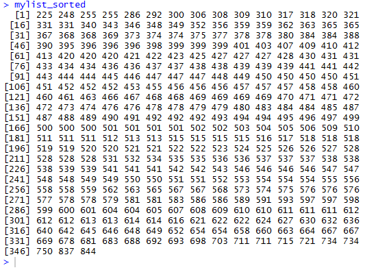
Table 5 presents, in the R style of presenting values, an ordered list of all 348 values. The 95^th percentile of these must be a value that has 95% of the values as less than this 95^th percentile value. But that means that we just have to find the value in the 95% of 348 position in the listing. 95% of 348 = 0.95*348 =330.6. Clearly, there is no item in position 330.6, but there is an item in position 330, namely 667, and there is an item in position 331, namely 669. Which value we choose, or what value around 668 we choose depends on which of those 9 different rules that we want to use. However, it is safe to say that nobody is really going to care all that much if we just choose 669 as being the 95^th percentile. As we will see later, if we were to ask R to compute the 95^th percentile it would give us the value 668.3.

How about finding the 40^th percentile? We just compute 40% of 348 = 0.4*348 =139.2. Again, there is no item in position 139.2, but there is an item in position 139, namely 476, and there is an item in position 140, namely 476. We could justifiably choose 476 as the answer, and R will also choose 476.

To find the 27^th percentile we compute 27% of 348 = 0.27*348 =93.96. There is no item in position 93.96, but there is an item in position 93, namely 444, and there is an item in position 94, namely 445. It would be reasonable to choose 445 as the answer. However, R will choose 445.69.

Quantiles vs. Percentiles

So far we have just talked about percentiles. The title of this page includes quantiles. What is the difference? Not much. Percentiles are given as percent values, values such as 95%, 40%, or 27%. Quantiles are given as decimal values, values such as 0.95, 0.4, and 0.27. The 0.95 quantile point is exactly the same as the 95^th percentile point.

R does not work with percentiles, rather R works with quantiles. The R command for this is quantile() where we need to give that function the variable holding the data we are using and we need to give the function one or more decimal values. Interestingly, the quantile() function returns the desired value but it does so with a name in the form of a percentage. We will look at an example.

First, we need to get the values in our table. The R command set.seed(34211) is used to set a starting point for the pseudo-random number generator that R uses. By setting the seed value we create an environment where the subsequent generation of seemingly random values is completely determined. That way, should we or someone else, want to replicate our steps, the random numbers we or they get will be exactly the same as the values we will see here. Figure 1 starts with that statement.

Figure 1

Figure 1 ends with a statement, mylist <- round( rnorm(348, mean=500, sd=100 ) ) that generates 348 random values such that those values will have a mean of approximately 500 and a standard deviation of approximately 100. Those 348 random values are then rounded to be 348 random integers. Finally, those values are assigned to the variable mylist.

Once defined, we can ask to see the values by using the mylist command. The result is shown in Figure 2.

Figure 2

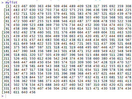
You will notice that he values in Figure 2 are identical to those in Table 2. In fact they are identical because the text in Figure 2 was copied and placed in this web page as the data behind Table 2.

There is no need to do the actions shown in Figures 3 and 4, but doing them allows us to verify the contents of Table 3. In Figure 3 we use the sort() function to sort the values stored in mylist. We assign those sorted values to the variable mylist_sorted.

Figure 3

Then, in Figure 4, we use the command mylist_sorted to display the entire sorted collection of values.

Figure 4

To actually find a percentile value for mylist we ask for the corresponding quantile by using the quantile() function. Figure 5 shows the command to get the 95^th percentile of mylist, along with the resulting value.

Figure 5

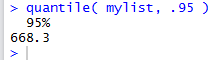
Note how the quantile(mylist,.95) command produces output that is actually labeled as 95%. The value is the same 668.3 that was noted above.

We could give quantile() more than one value by using the c() function to combine those values into one argument as in quantile(mylist,c(.95,.40,.27)), the statement shown in Figure 6.

Figure 6

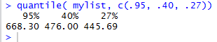
As you can see, the statement produces the percentile values that we expect.

We could take the idea of giving quantile() many values to a higher level. The statement quantile(mylist,seq(0.05,0.95,0.05)) asks R to compute percentile values for 5%, 10%, 15%, and so on up to 95%. The command and its related output are shown in Figure 7.

Figure 7

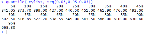
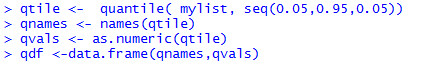
The output in Figure 7 gives us all of the values that we requested. However, it might be nice if we could convert this to a vertical format. The statements shown in Figure 8 recompute the percentiles that we just found, but store the results in the variable qtile. Then, the statements pull out the names and the values in qtile, concluding with the creation of a data frame, that is then stored in the variable qdf.

Figure 8

Then, the statement qdf produces the vertical listing we desired.

Figure 9

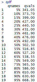
Of course, the labels on the top of the values come from the names of the variables we used to create the data frame. We can use the names() function to change those titles to something more appropriate. This is done in Figure 10.

Figure 10

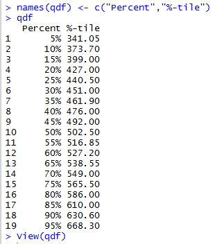
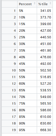
Now that the data frame is defined we can use the View(qdf) to produce the "pretty" output shown in Figure 11.

Figure 11

The work that we have seen so far has fallen into the form: Here is a list of data values, now find the n^th percentile of that data (using the quantile() function). We can, and often do, turn that question around. For example, with the data given in Figure 4, we might ask "What percentile is the value 432?" That is an especially nice value because 432 is not a value in Figure 4. Remembering that the values in Figure 4 are already sorted, we can see that there are 75 values that are less than 432. Therefore, since there are 348 values in the table, it makes sense to say that 75/348 ≈ 0.2155 or 21.55% of the values are less than 432, or that 432 is the 21.55 percentile.

This gets more complicated if the value we are using is in the table, and especiallycomplicated if the value is repeated in the table. For example, what percentile should we assign to 528? There are 209 values less than 528 but 528 occupies positions 210, 211, 212, and 213 of the sorted list. As we might expect, there are any number of "rules" that might guide us to an answer for this kind of situation. Because there is no definitive universally accepted rule, we can come up with one that serves our purpose. Our rule will give an answer that, in all but the most contrived situations, will be close to the answer that any of the other generally accepted rules produce. Our rule is captured in the function find_percentile(). We need to give that function the list of values (it does not even have to be a sorted list) and the value for which we want to determine a pecentile. Thus the statements

 source( "../find_percentile.R") 
 find_percentile( mylist, 432)
 find_percentile( mylist, 528)
 find_percentile( mylist, 562)

will return the percentile to be assigned to the values 432, 528, and 562. This is shown in Figure 12.

Figure 12

Here is a listing of the R statements used on this percentage

# for the percentile web page
set.seed(34211)
mylist <- round( rnorm(348, mean=500, sd=100 ) ) 
mylist 
mylist_sorted <- sort( mylist )
mylist_sorted
quantile( mylist, .95 )
quantile(mylist,c(.95,.40,.27))
quantile(mylist,seq(0.05,0.95,0.05))
qtile <- quantile(mylist,seq(0.05,0.95,0.05))
qnames <- names(qtile)
qvals <- as.numeric(qtile)
qdf <- data.frame(qnames,qvals)
qdf
names(qdf) <- c("Percent","%-tile")
qdf
View(qdf)
source( "../find_percentile.R") 
find_percentile( mylist, 432)
find_percentile( mylist, 528)
find_percentile( mylist, 562)

Table 1
Quartile Name	Percent of Values Less Than the Quartile Value
Q₁	25%
Q₂	50%
Q₃	75%