One Population; Paired Samples

Return to Topics page
There are many situations in which we get values from a sample, have some "intervention" with the sample, and then get new values from that same sample. If we have identified the earlier and later values with particular members of our sample, then we can look at the difference between values for each member of the sample.

For example, we start with a population. From that population we take a sample of members. We take a measurement on each of those members, and we associate that measurement with its particular member. Then we conduct some intervention on the members. That is, we do something to or allow something to possibly change the characteristic that we are measuring. Later, after the intervention, we take a new measurement on the same members of the same sample.

As a particular example, we have a sample of 25 students from the college. We administer a test to these 25 students. The result of the test is a number between 20 and 40. We record the test result of each of the 25 students. Then we show the students a video. After the video, we administer the same test to those 25 students, and we record the new score for each student. Table 1 shows the results of this experiment. For each student the Early measurement is paired with the Later measurement.
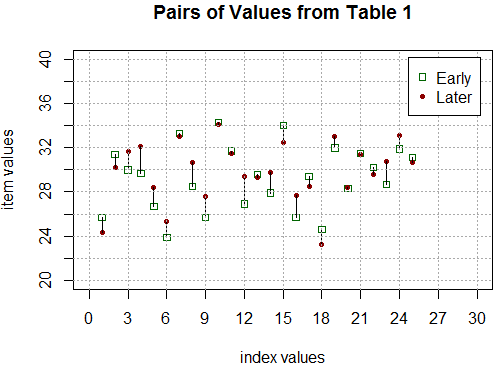
We could plot these pairs of values as shown in Figure 1. In that plot the pairs of values are shown above each of the index values and a line connects the paired values.

Figure 1

Our interest is not with the values themselves but rather in the change in values. That is, for each student we want to see the change in the value. That means that we want to find the 25 "Later"-"Early" values. Those values are shown in Table 2.
But now, instead of having two separate lists of values, we have just one list of values. We can use that list as a sample of the difference between scores across the population if we had measured the population early, done the intervention on the entire population, and then, later, measured the population again. That means that we can use the sample values to generate a confidence interval for the difference of the scores across the population and/or we can test the null hypothesis that the difference is zero versus an alternative hypothesis (the difference is not zero, the difference is less than zero, or the difference is greater than zero). But once we have resolved the original two lists into the one list of Table 2 then we are looking at building a confidence interval or testing a hypothesis based on that one list. That is a task that we solved earlier.

In our example we can generate the values, find the difference, and then create a confidence interval (we will use a 95% confidence level) via the following R commands.

source("../gnrnd4.R")
gnrnd4( key1=1293112410, key2=330003200298 )
L1
L2
L3 <- L2-L1
L3
source("../ci_unknown.R")
ci_unknown(s=sd(L3), n=length(L3),
           x_bar=mean(L3),
           cl=0.95)

The console version of those commands is shown in Figure 2.

Figure 2

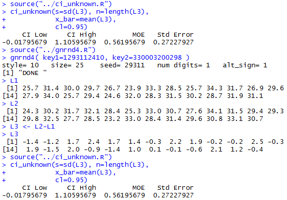
From Figure 2 we see that the 95% confidence interval for the difference of the scores is (-0.018,1.106).

Having defined L3 we could test H₀: d=0 against the alternative hypothesis H₁: d≠0 at the 0.05 level of significance via the commands

source("../hypo_unknown.R")
hypoth_test_unknown(
  0,  0, sig_level=0.05,
  length(L3), mean(L3), sd(L3))

Figure 3 shows the console view of those commands.

Figure 3

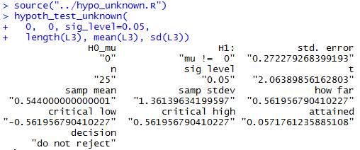
From Figure 3 we see that the mean of the differences was 0.544, a value that is between the two critical values, -0.562 and 0.562 causing us to not reject the null hypothesis via the critical value approach. Or we see that the attained significance with 24 degrees of freedom is only 0.0572, which is not less than the 0.05 level of significance set in the statement, so we do not reject the null hypothesis via the attained significance approach.

You may have noticed that this topic is presented in the middle of a sequence of topics dealing with samples from two populations. Here, however, we end up dealing with one list of data values, the differences between paired sample values. To do this, once we had the problem resolved to our one list of values, we just returned to the concepts and commands that we had developed for dealing with one population samples in order to get a confidence interval and/or a test on the null hypothesis that the differences are zero. Why, then, is this topic placed here?

One reason to do it here is that we start with what seems to be two samples. However, those values are paired, and our interest is in the change in the values within each pair, not in the values themselves. Another reason is that we generally look to see if that change is different from zero, in the same way that we have been looking, in the previous two topics, to see if the difference in those means is zero. Therefore, it is almost a "tradition" to place this topic within the discussion of two sample topics.

Let us look at a second example before we leave the topic. Here we have 32 pairs of samples. We have a "before" and "after" score for each member of the sample. We want a 98% confidence interval for the difference in the scores, where we understand that difference is the growth of the values from "before" to "after". In addition, we want to test, at the 0.02 level of significance, the hypothesis H₀: d = 0 against the alternative H₁: d > 0. You might note that the confidence interval will spread the 2% across both ends of the interval whereas the test will be a 1-sided test with the 2% just at the top.

The pairs of sample values are given in Table 3.
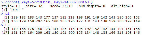
To generate and confirm these samples we will use the commands

gnrnd4( key1=572193110, key2=140002800163 )
L1
L2

The console result of those commands is in Figure 4.

Figure 4

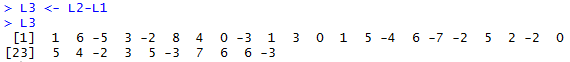
We want to resolve these to one list of differences within the pairs. To show the "growth" in values we want to find "After"-"Before". The commands

L3 <- L2-L1
L3

do this. Their console view is in Figure 5.

Figure 5

To find the confidence interval for the values now in L3 we could find the length of L3 (which we know to be 32), the mean of L3, and the sample standard deviation of L3, along with the t-value for 31 degrees of freedom that has half of the area outside of the 98% confidence interval above that value, and then we could compute the confidence interval. Alternatively, we can have R do all of this with the command

ci_unknown(s=sd(L3), n=length(L3),
           x_bar=mean(L3),
           cl=0.98)

which produces Figure 6.

Figure 6

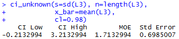
From Figure 6 we get the 98% confidence interval (-0.213,3.213).

To run the hypothesis test we continue with the command

hypoth_test_unknown(
  0,  1, sig_level=0.02,
  length(L3), mean(L3), sd(L3))

which gives the result shown in Figure 7.

Figure 7

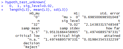
from which we get the one, high, critical value, 1.497, and the sample mean, 1.5, resulting in a decision to Reject H₀ in favor of H₁. And we get the attained significance, 0.0198, which, since it is less than our 0.02 level of significance, results in the decision to Reject H₀ in favor of H₁.

Finally, just so that we can see the changes from L1 to L2 we can use the statements

plot(1:32,L1, col="darkgreen",
     xlim=c(0,40), xaxp=c(0,40,10),
     xlab="index values",
     ylim=c(110,230), yaxp=c(110,230,12),
     ylab="item values",pch=22,
     main="Pairs of Values from Table 3"
)

points(1:32,L2, col="darkred", pch=20)
for(i in 1:32)
{ lines(c(i,i),c(L1[i],L2[i]))}
abline(h=seq(110,230,10),lty=3,col="darkgray")
abline(v=seq(0,40,4),lty=3,col="darkgray")
legend("topright", 
       legend = c("Before","After"),
       pch=c(22,20),
       col=c("darkgreen","darkred"),
       inset=0.03)

to generate the plot shown in Figure 8.

Figure 8

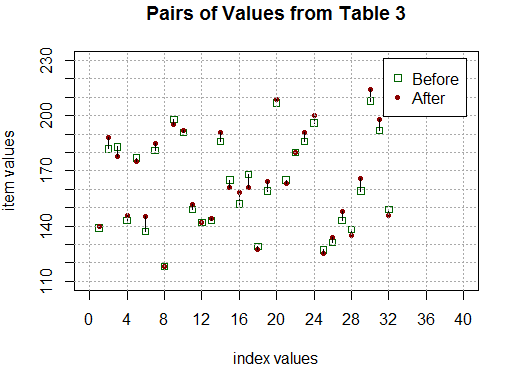
Figure 8 shows us that sometimes the scores go up, as in item 6,

, sometimes the scores go down, as in item 17,

, and sometimes the scores do not change much at all, as in item 22,

. However, overall, there are more ups and further ups than downs. With the mean of L3 being 1.5, we see that the average increase in the sample was 1.5. Furthermore, there is enough of an average increase, given the sample size and the sample standard deviation, for us to say, at the 0.02 level of significance, that we have enough evidence to reject the idea that the intervention, if applied to the population, would not change the scores in favor of the alternative that the average scores would go up.

Return to Topics page
©Roger M. Palay Saline, MI 48176 February, 2016