Our File Convention
Return to Topics page
In this course we will be using RStudio to run R statements.
At the same time, we will want to have access to the numerous files that I have
created for this course. These files are available on my web site and they are
available on the USB drive that was handed out to each student.
From within an RStudio session we want to have easy access to those files.
The command that we will use to load a file into our environment is the
source() command. We give the source()
command the location of the file that we want to load.
Access the file from the web
One way to load the
gnrnd4.R file would be to give the command
source("http://courses.wccnet.edu/~palay/math160r/gnrnd4.R")
This loads the file directly from my web site.
This method will work, as long as we have internet access and as long as
my web site remains available.
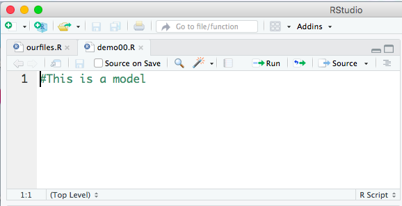
In fact, Figure 1 shows the RStudio editor version of that statement.
Figure 1
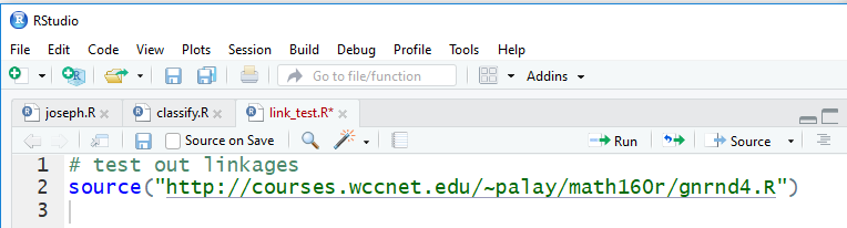
If we run that statement in Figure 1 we see
the R execution of the statement in Figure 2.
Figure 2

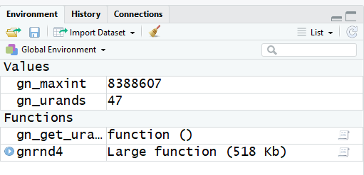
About the most that can be said from looking at Figure 2
is there were no errors. However, if we look at the
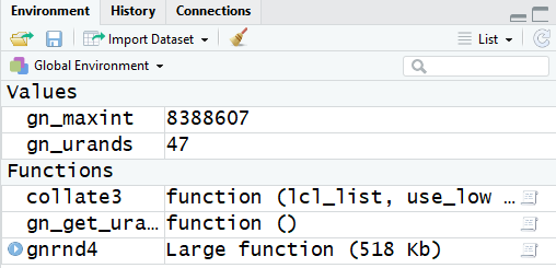
Environment pane, shown in Figure 3, we see that
the function gnrnd4() has now been loaded into
our environment, meaning that it is now ready to use.
Figure 3
Although the statement
source("http://courses.wccnet.edu/~palay/math160r/gnrnd4.R")
works
it is really a lot to write just to load that one function.
Furthermore, in this course we will be loading many functions and
many of those will be loaded numerous times. Therefore, it would be nice if we had
an easier way to load them.
Access the file from the USB drive
One way would be to give each student a USB drive with all of the files for the functions
on that USB drive. In fact, this is done in my classes. Once a student has such a drive they can
plug the drive into their computer and then access the files directly from the USB drive.
This is done slightly differently on a PC than it is on a Mac.
I have plugged a USB drive for this course into the PC on which this page is
being written. On my PC whenever a new USB drive is plugged in the computer responds
by opening the file explorer to show that new drive. [On other PC's you may need to specifically as
the computer to open the file explorer to look at the files on the newly installed
drive.]
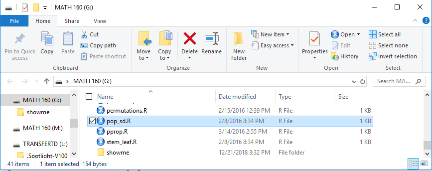
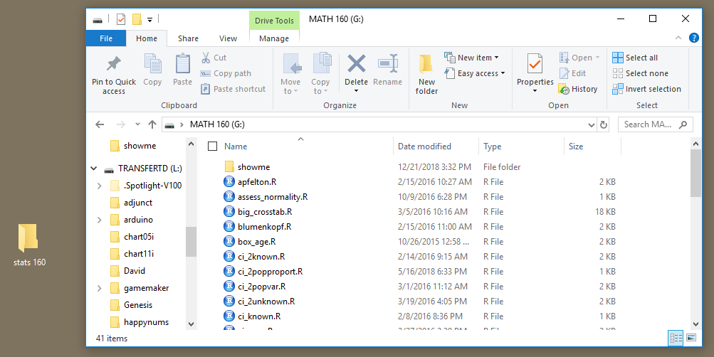
Figure 4 shows that file explorer display.
Figure 4
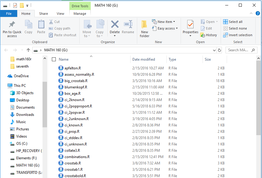
Note, that Figure 4 shows, in two places, that this drive has been assigned the drive letter G for this
installation. Therefore, we could load the file collate3.R
by using the statement
source("G:collate3.R")
This is shown in the editor in Figure 5.
Figure 5

When we execute that statement from Figure 5 we get the
console output shown in Figure 6.
Figure 6
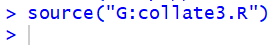
That shows no errors. Furthermore, if we look in the
environment pane we see that collate3()
is now a defined function.
Figure 7
This looks like a nice approach, at least on a PC. However, it has one serious drawback.
That is there is no certainty that the next time I plug this USB drive into even this computer we
will find that it has been assigned the drive letter G. One of our goals is to have a process,
the commands written into our editor file and later saved, that is repeatable with no need to
change the text of the file! Having to change every source() statement to
reflect a newly assigned drive letter violates that goal.
Before we move on, let us step back and look at the steps that we would need to do on a
Mac in order to access a file from the USB drive.
When I plug my USB drive into a Mac, after a moment or two, the icon for that drive
shows up on my desktop, as shown in Figure 8.
Figure 8
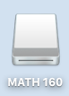
It is clear from Figure 8 that the name of the USB drive is MATH 160.
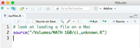
If we are running RStudio on a mac then the command to load the file ci_unknown.R
from that USB drive is
source("/Volumes/MATH 160/ci_unknown.R")
That is shown in Figure 9 as the command in the editor.
Figure 9
If we run that command then it is shown in the console, as illustrated in Figure 10.
Figure 10
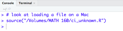
There is no error message in the console so we can assume the
command was successful. We can confirm that by looking at the
Environment pane, shown in Figure 11.
Figure 11
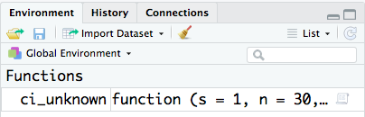
There we see that ci_unknown() is now
defined in our environment.
In one sense the Mac approach is better than the PC approach because unless we change the
name of the USB drive we will always, on a Mac, be able to reference the ci_unknown.r
file on it via the statement
source("/Volumes/MATH 160/ci_unknown.R")
However, we cannot take that script (the file of our commands) and run it on a PC because the PC does not
recognie the Volumes name, nor does it recognie the MATH 160 name. The PC wants
the drive letter, not those names.
We want some method that allows our commands to be run without change each time we
move our script to a new computer.
R, and therefore RStudio, always looks for files in its working directory.
The working directory is, by default, the directory from which we start our RStudio, and therefore our R,
session. On the PC used in the early figures I started RStudio from the desktop.
That meant that the working directory was
C:/Users/Roger.touchscreen/Documents
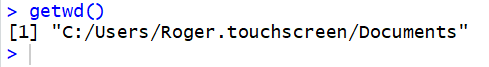
You can use the command getwd(), in the console, to have R
display the working directory. That is shown, for the PC, in Figure 12.
Figure 12
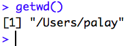
On the other hand, on the Mac, even though I started RStudio from the desktop
the working directory
turns out to be
/Users/palay
and, again, we can get that from typing the getwd() command in
the console, as shown, for the Mac, in Figure 13. [By the way, getwd() is the
built-in function in R for "get the working directory".]
Figure 13
Once again, we want to structure our scripts, our sequences of commands, such that when we take the
scripts from one computer to another we do not need to change the scripts in order to
have them work properly. Certainly, if we were to use the approach
demonstrated back in Figure 1 then we would meet our primary goal, as long as we have internet access.
However, we know that the command in Figure 1 was just to awkward and long.
And, we know that unless we specify otherwise, R will look for the
command file in the working directory. We have seen that we could specify
otherwise, on a PC, by using G:filename.R or, on a Mac,
by using /Volumes/MATH 160/filename.R. The problem with this approach is that we cannot be sure it will be
drive letter G on a PC and our scripts would have to change if we moved from
PC to Mac or Mac to PC.
Access the file from a subdirectory on the USB drive
Here is a slightly different approach. If we put our script in a subdirectory (subfolder)
of our USB drive, then all of the files that I provided on that drive will
be in the parent directory of the script. For example, if we create a directory (folder) called showme
on the USB drive, and if we somehow, get our script into that folder, then we could start
RStudio by clicking on the script name. The result of that would be twofold.
First, the working directory would be the our showme directory on our USB
drive.
Second, all of my files would be in the parent directory.
Let us look at the PC first.
I have taken the USB drive and created the showme subdirectory in it.
This is shown in the file explorer listing shown in Figure 14.
Figure 14
In Figure 14 you can see the new subdirectory (subfolder) called
showme. We could double click on that icon to
look at the contents of showme. That is what was done
to move to Figure 15.
Figure 15
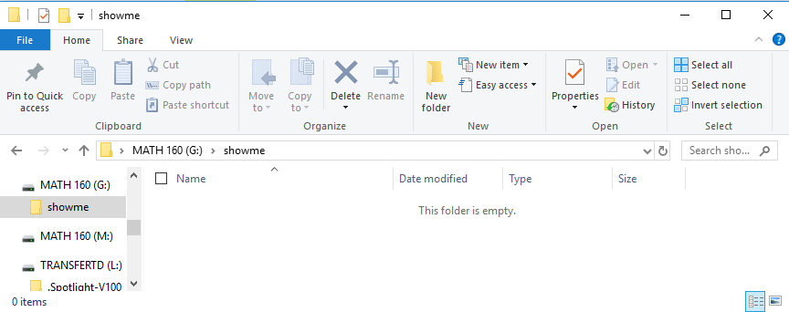
As expected, the subdirectory is currently empty. That is not what we want.
We want to have a script in here so that we can
click on the script to open RStudio.
There are many ways to create such a script.
We will use the method of finding a script somewhere else, copying it,
and then pasting the copy here.
The script we want is back in the "parent" directory, the directory listing we saw back in Figure 14.
We return there, as shown in Figure 16, and find the file model.R.
Figure 16
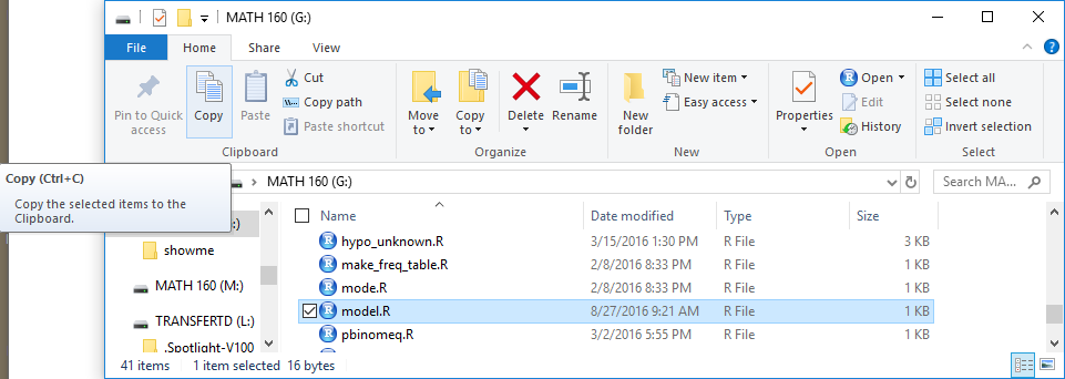
Once we highlight the file in Figure 16 we copy it and then return to our subdirectory,
showme, where we paste the file. Now, in Figure 17, we have a copy of model.R
in our subdirectory. Rather than leave it with that name, we will rename the file.
Figure 17
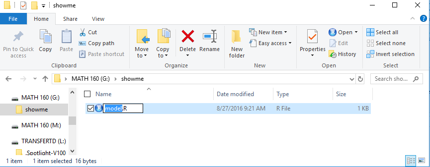
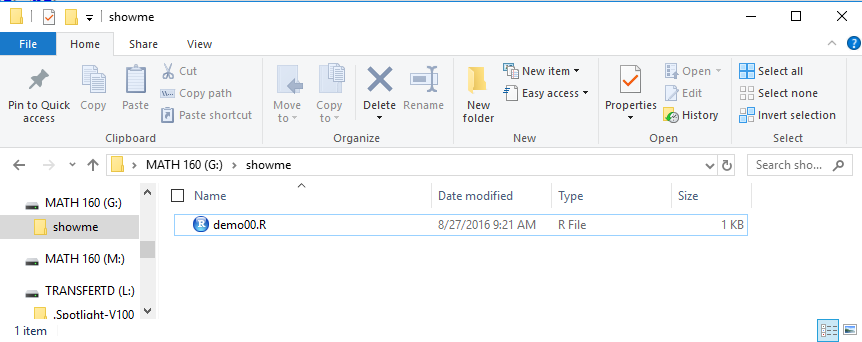
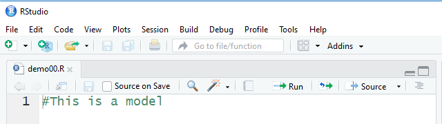
Figure 18 shows the file, renamed as demo00.R.
Figure 18
Before going on we will demonstrate the same tasks on a Mac.
To get to Figure 19 on my Mac I double clicked on the MATH 160
icon, the one we saw back in Figure 8. That opened Finder to show all
of the files in that directory (folder).
Then I created a new folder and called it showme.
The result is shown in Figure 19.
Figure 19
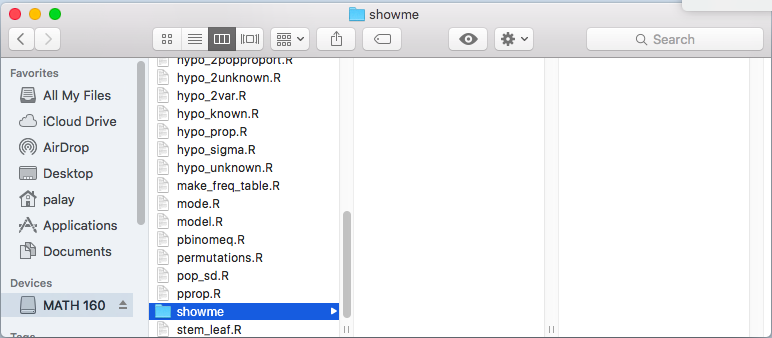
In the Mac, once the showme folder name is highlighted,
the pane to the right of the file list shows the contents of that folder.
Figure 19 has a blank pane there showing that, as we would expect,
our new folder is empty.
We want to get a script into that folder.
Our approach to thi will be to copy the file model.R
from our main MATH 160 directory to the showme
directory.
To start doing this we highlight the model.R name in our
MATH 160 directory, as shown in Figure 20.
Figure 20
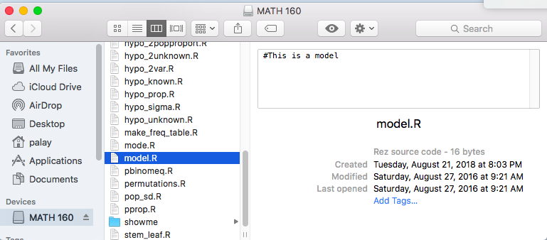
You might notice that when we highlight the model.R name
Finder, as best it can, the contents of the file and some additional information
about it.
We will copy the file, then move to highlight and open our showme
subdirectory, and then paste the file into the pane that shows the contents of
the subdirectory, i.e., the pane to the right of the file name list.
This result is shown in Figure 21.
Figure 21

It will be inconvenient and confusing to keep the name of this file model.R.
Instead we highlight the name and then rename it, in this case to demo00.R
as shown in Figure 22.
Figure 22
Again, because the ile name demo00.R is highlighted Finder
displays the contents of the file for us the the next pane to the right.
After Figure 22 we are in the same place on a Mac that we were after
Figure 18 on a PC. In either case we have accomplished our goal, namely
we have created a script in a subdirectory just below the all of the files that I have supplied.
That means that if we start RStudio from our newly created script the working directory
will be showme. Furthermore, we can tell RStudio that
any file that we want to load is just "up one directory" from the working directory.
We will now demonstrate this, first on the PC (figures 23 through 31)
and then on the Mac (figures 32 through 44).
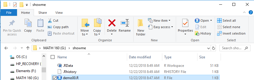
Back in Figure 18 we had the demo00.R file
displayed in the file explorer. There are two possible cases to consider.
The first is that we have already associated
files with the .R extension with the RStudio
application. We can recognize that by seeing the RStudio icon just to
the left of the file name, as it is in Figure 18.
In that case, we can just double click on the file name to open RStudio
as shown, in part, in Figure 23.
The second case, where the file is not associated with the
application, should only happen once as the next step solves that
issue henceforth. If the RStudio icon is not to the left of the file name
then
- right click on the file name
- select the "open with" option
- highlight the RStudio option
- make sure the "Always use this app to open .R files" box is checked
- click on OK.
This will open RStudio and take us to Figure 23.
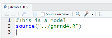
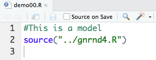
Figure 23 shows the editor pane in an RStudio run. We see that the
contents of the demo00.R file are displayed in Figure 23.
We also note that there is a second tab, link_test.R that
is available. That is left over from an earlier run of RStudio.
We do not want to clutter our display with that tab.
Therefore, we can click on the x on that tab
to remove it. This yields Figure 24.
Figure 23
The editor in RStudio allows us to create scripts that we can save and rerun
at a later time.
Figure 24
We will add the line
source("../gnrnd4.R")
to that editor listing.
The ../ indicates that the program is to look in the
parent directory to find the file.
Since the working directory is our subdirectory showme,
the parent directory will be our USB drive main directory.
It is the location of all of the files that I have
supplied.
This is shown in Figure 25.
Figure 25
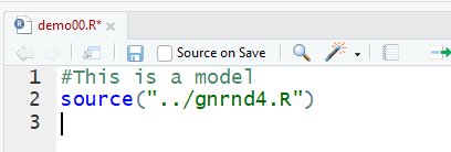
Not only does Figure 25 show that new line, but we notice that the name
demo00.R on the tab has changed to red.
That indicates that we have changed the file but that we have yet to save the changes.
If we put the cursor back on our new line,
or if we highlight our entire new line,
and then click on the  icon at the
top of the editor pane, then RStudio will send that line to be executed by R
with the statement and its result showing in the console pane, shown in Figure 26.
icon at the
top of the editor pane, then RStudio will send that line to be executed by R
with the statement and its result showing in the console pane, shown in Figure 26.
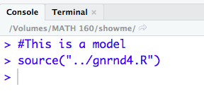
Figure 26
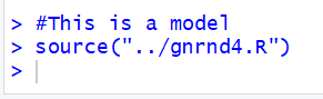
There is not much to see here, in Figure 26, because the
command executed perfectly with no errors.
Instead, to see that something really happened we
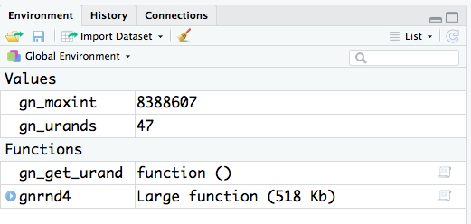
look at the environment pane, shown in Figure 27.
Figure 27
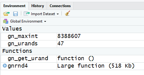
We can see that the file has actually loaded and that the function gnrnd4()
is now available.
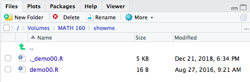
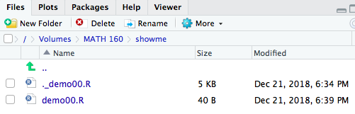
A quick look at the Files tab in the lower right pane of the
RStudio window appears in Figure 28
Figure 28
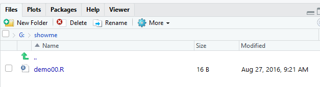
There we can see that the demo00.R file is listed as the
only file in our subdirectory.
If we return to the editor pane and click on the save icon,
 , we can see that the file name on the tab returns to
black in Figure 29.
, we can see that the file name on the tab returns to
black in Figure 29.
Figure 29
Then we can return to the Files tab in the lower right pane,
in Figure 30, and we can see that the new size and file date reflect the
newly saved version of the file.
Figure 30

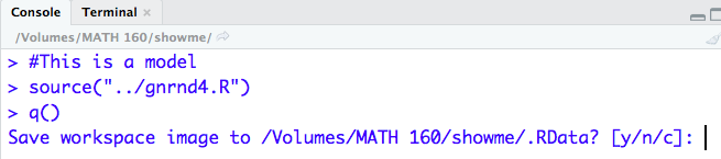
Finally, to quit our session we return to the
console pane and give the command q(),
press the Enter key, and then respond to the prompt with a y,
followed by another Enter key. That ends our session, and it
saves two "hidden" files in our working directory.
We can see them, on a PC, by returning to the file explorer
shown in Figure 31.
Figure 31

The .RData file holds the environment.
The .Rhistory file holds a list of the commands that we gave during
this and any previous sessions using this subdirectory as the working directory.
Figure 32
What we have seen in Figures 23 through 31 is a scheme for
creating scripts that allow us to reference the files that I provided via a simple and consistent
reference to "look in the parent directory" and we do this via the
../ prefix to the file name in our source()
command.
We can do the same thing on a Mac.
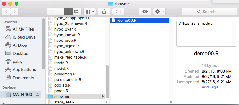
Figure 33 shows the Finder listing of our
demo00.R file.
Figure 33
There are two possible cases here.
The first is that we have already associated
files with the .R extension with the RStudio
application. We can recognize that by seeing the RStudio icon just to
the left of the file name.
In that case, we can just double click on the file name to open RStudio
as shown, in part, in Figure 34.
The second case, where the file is not associated with the
application, should only happen once as the next step solves that
issue henceforth. If the RStudio icon is not to the left of the file name
then
- click on the "options" icon,

- select the "open with" option
- select Other..., do this even if RStudio is an option
- this brings up a list of applications, find and highlight
RStudio in that list
- highlight the RStudio option
- make sure the "Always open with" box is checked
- click on OPEN.
This will open RStudio and take us to Figure 34.
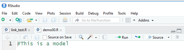
Figure 34 shows the editor pane in an RStudio run.
We see that the contents of the demo00.R file are displayed in Figure 34.
We also note that there is a second tab, ourfiles.R that is available.
That is left over from an earlier run of RStudio.
For now we will just leave it there.
Figure 34
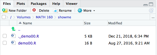
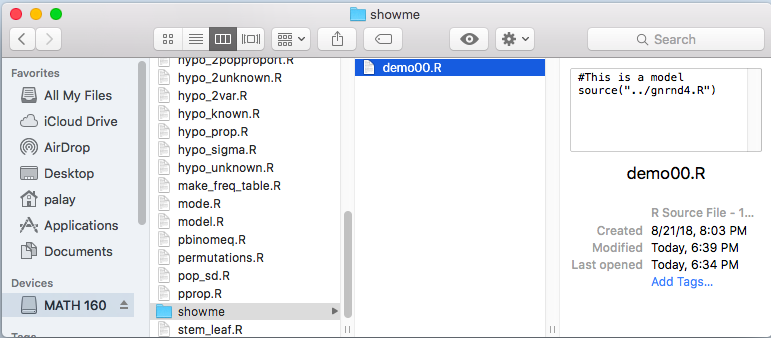
A quick glance at the Files tab in the lower
right pane of our RStudio session shows our demo00.R
file, along with its creation date, and it shows another file,
._demo00.R which is a hidden file (though not hidden to RStudio)
that the Mac uses for its own purposes.
Figure 35
Returning to the editor pane
we will add the line
source("../gnrnd4.R")
to that editor listing.
The ../ indicates that the program is to look in the
parent directory to find the file.
Since the working directory is our subdirectory showme,
the parent directory will be our USB drive main directory.
It is the location of all of the files that I have
supplied.
This changed script is shown in Figure 36.
Figure 36
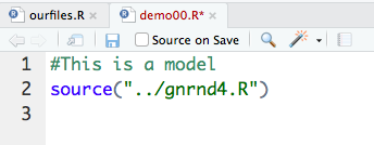
Not only does Figure 36 show that new line, but we notice that the name
demo00.R on the tab has changed to red.
That indicates that we have changed the file but that we have yet to save the changes.
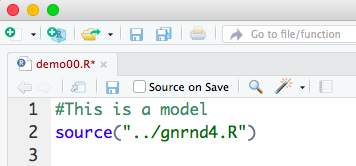
Before we look away from the editor, this is a good time for us to
close down the ourfiles.Rtab.
To do this we just click on the x
on that tab. We can see in Figure 37 that the tab has been closed.
Figure 37
If we put the cursor back on our new line,
or if we highlight our entire new line,
and then click on the icon at the
top of the editor pane, then RStudio will send that line to be executed by R
with the statement and its result showing in the console pane, shown in Figure 38.
Figure 38
There is not much to see here, in Figure 38, because the
command executed perfectly with no errors.
Instead, to see that something really happened we
look at the environment pane, shown in Figure 39.
Figure 39
We can see that the file has actually loaded and that the function gnrnd4()
is now available.
A quick look at the Files tab in the lower right pane of the
RStudio window appears in Figure 40
Figure 40
We have not saved our changed editor file so there is no change in these files.
If we return to the editor pane and click on the save icon,
, we can see that the file name on the tab returns to
black in Figure 41.
Figure 41
Then, we look at the Files tab in the lower right pane,
shown in Figure 42.
Figure 42
Both our file, demo00.R and its Mac companion hidden file,
._demo00.R have been updated.
Figure 43
Then we return to the console pane where we end our session
by typing the command q() , pressing the Return key, getting the
prompt, then typing y and pressing Return again.
That will end our RStudio session.
We look back at our Finder window, shown in Figure 44.
Figure 44
There we see that our file, demo00.R is saved, with its new contents
and new date and time for its Modified attribute.
Those who did not skip over the previous discussion of doing this same thing
on a PC might notice that the two hidden files, shown for the PC version in Figure 32,
namely, .RData and .Rhistory do not show up here.
They are actually present in the Mac version but Finder does not display
hidden files. We would see those files in a new RStudio session if we opened
our session from the showme subdirectory.
What we have seen in Figures 33 through 44 is a scheme for
creating scripts that allow us to reference the files that I provided via a simple and consistent
reference to "look in the parent directory" and we do this via the
../ prefix to the file name in our source()
command.
Move the files to the computer; access them from a subdirectory
The beauty of using the USB and subdirectories on it is that
your work is completely portable. Furthermore, we have the advantage of being able to reference
my files via the simple ../ prefix for the file name, as in
../gnrnd4.R.
The ugly part of this scheme is that USB drives are easy to lose and easy to damage.
An alternative is to use the USB once in order to copy my files and place them
into a directory on your computer. In that way you can create subdirectories in the directory holding my files and
you do not need to plug in the USB drive again. You lose the quick portability but maintain
the ease of referencing my files.
We will do this first on the PC (Figures 45-51) and then again
on the Mac (Figures 52-70).
In both cases we will create our new directory on our desktop.
This location is not a requirement but it does ease the process.
On the PC, identify an open area on the desktop
and right click at that point.
This will open the left box shown in Figure 45. Then move down to the New
option and that will open the right box.
Figure 45
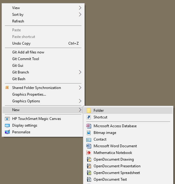
Click on the Folder option shown in Figure 45.
This creates a new directory on the desktop, shown in Figure 46.
Figure 46

We do not want the default name so we type a new name, in this case
stats 160 as shown in Figure 47.
Figure 47

Next open the file explorer to look at the USB drive (plug it in first if need be).
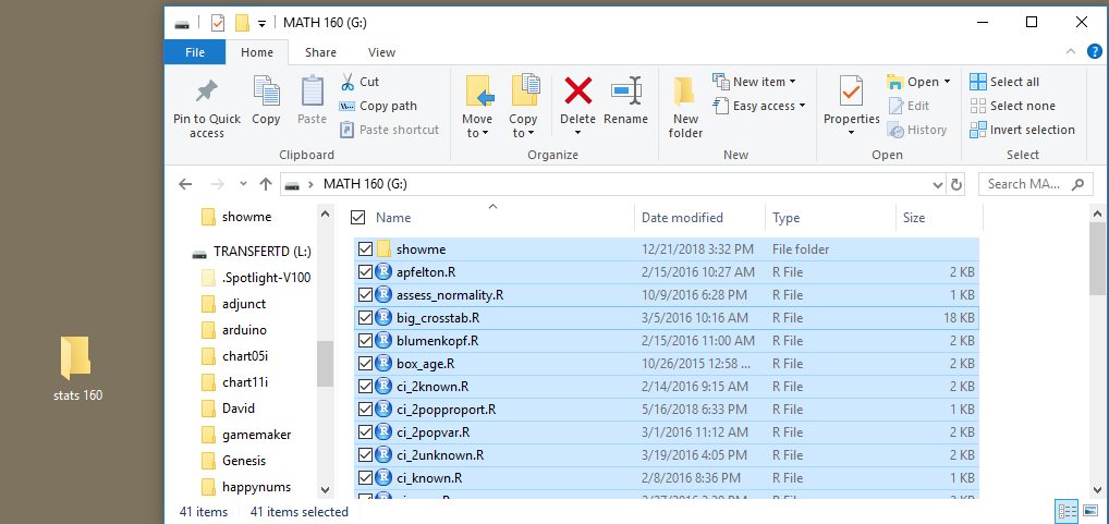
Figure 48
Now, press CTRL-A to select all of the files. Note that in this case we are using the
USB on which we did our earlier work so it includes our previously
created showme
subdirectory. There is no problem copying that too.
Figure 49
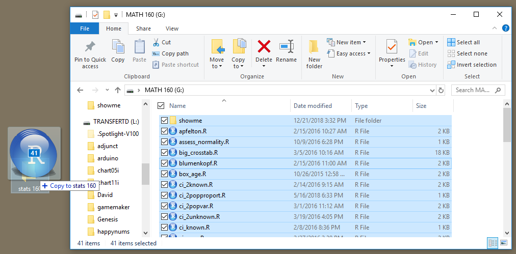
Once all the files are highlighted, just point to the highlighted area and drag
that over the newly created directory. Then drop the files in that directory.
Figure 50
Once that is done we can double click on the new stats 160
directory and the computer will open a file explorer window
for us to see the files in the directory.
Figure 51

At that point we are ready to go. If we had a new project we would
- create a new subdirectory here
- rename that newly created subdirectory
- copy the
model.R file
- open the new subdirectory
- paste the copy of the
model.R file
- rename that newly created file
- double click on the file to start a new RStudio session with the new file
open in the editor.
Now, let us do the same thing on a Mac.
Find an open spot on the desktop and right click on it.
That opens the window shown in Figure 52.
Figure 52
Click on New Folder.
That creates a new filder on your desktop.
Figure 53
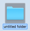
The default name of the folder will be something like untitled folder.
Change that to something more meaningful, in our case I chose stats 160
as shown in Figure 54.
Figure 54

Double click on the USB drive icon to
open the Finder page shown in Figure 55.
Figure 55
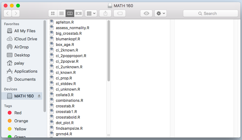
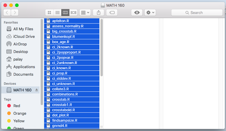
Select all the files in the USB drive. I used the Command-A sequence to do this.
Figure 56
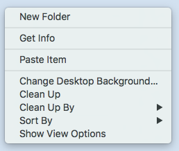
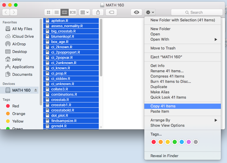
While pointing to the highlighted files, right click to open the
options list shown in Figure 57. There select Copy 41 items.
Figure 57
Double click on the new folder, stats 160,
that we created. This opens a Finder window similar to the one shown
in Figure 58.
Figure 58
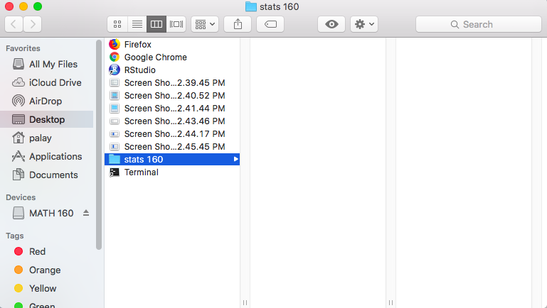
Be sure that the stats 160 item is highlighted
and click on the options icon to open the list shown in Figure 59.
Figure 59
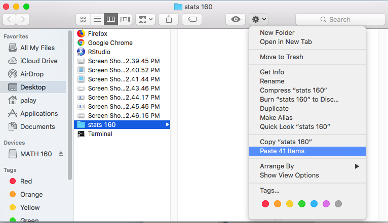
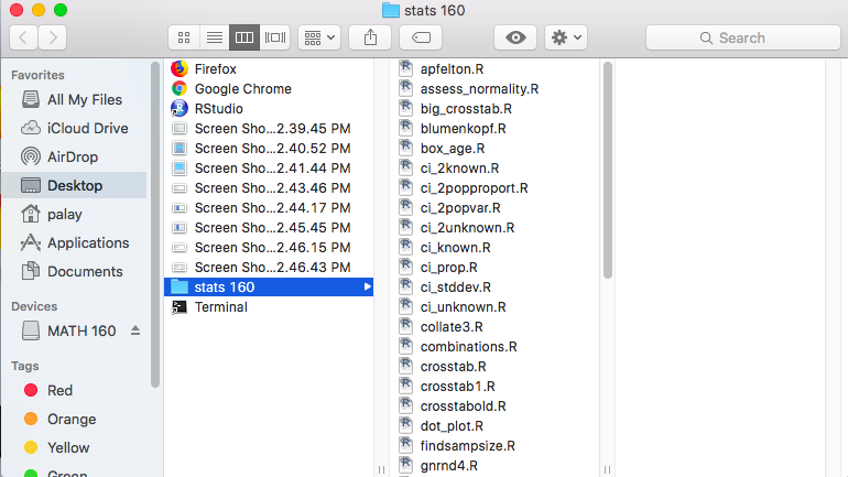
Select the Paste 41 items option. Once the items have been pasted the
files should appear in the stat 160 folder, as shown in Figure 60.
Figure 60
At that point we are ready to go. If we had a new project we would
- create a new subdirectory here
- rename that newly created subdirectory
- copy the
model.R file
- open the new subdirectory
- paste the copy of the
model.R file
- rename that newly created file
- double click on the file to start a new RStudio session with the new file
open in the editor.
In fact, let us do most of this. We click on the Options icon
to get the list shown in Figure 61.
Figure 61
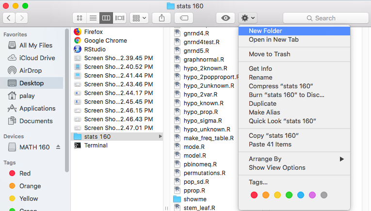
Click on New Folder.
Figure 62
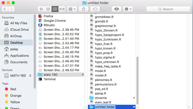
In Figure 62 we see the new folder is called untitled folder.
Figure 63
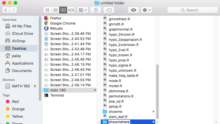
That is a bad name to leave so we will rename it, in this case we chose
showmehere. Then we went back to highlight model.R
and then right clicked on that name to open the options menu shown in Figure 64.
Figure 64
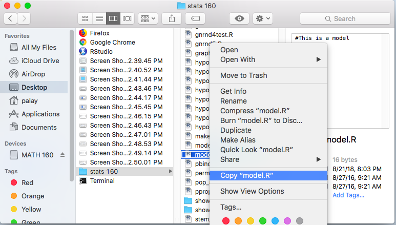
There we selected Copy "model.R.
Then, we clicked on the showmehere folder.
Figure 65
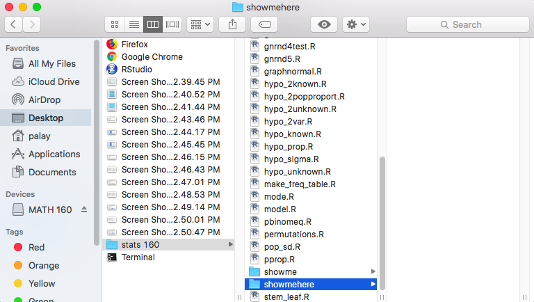
Clicking on the Options icon opens the list of options shown in Figure 66.
Figure 66
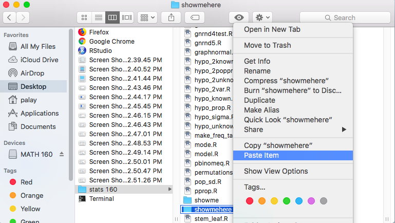
Select the Paste item option.
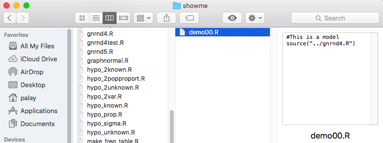
In Figure 67 we can see that the copy of the file is now in
the showmehere subdirectory,
but it still has the name model.R.
Figure 67
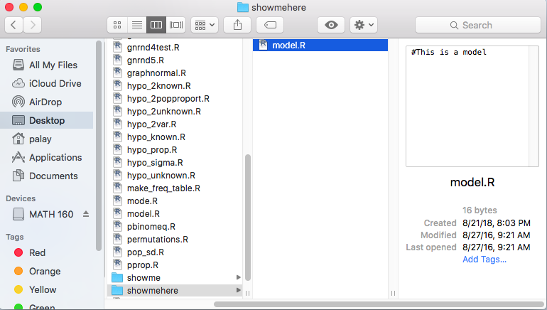
Then highlight that file, as in Figure 68.
Figure 68
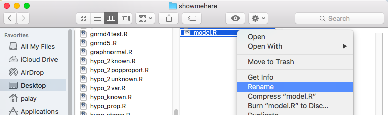
Select the Options icon to open the list of options shown in Figure 69.
Choose the Rename option.
Figure 69
We chose to rename the file demo01.R as shown in Figure 70.
Figure 70
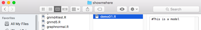
At this point we could double click on that file name
in order to open a RStudio session with demo01.R in
the editor and with the working directory being showmehere
which, in turn, makes the parent directory be stat 160 which holds all of the files
that I supplied on the USB drive.
Return to Topics page
©Roger M. Palay
Saline, MI 48176 January, 2019