Mac File Association Demo

Return to Topics page
This page displays the steps for the first time that we use RStudio for class work. When stalled RStudio, we actually started it from an icon on the desktop. That works, but it has some consequences that we do not want to encounter. Therefore, we have this alternative.

For this class you have been given a USB thumb drive. It contains many files that you will need for this class. It will be beneficial if we all use the USB drive the same way. On a Mac we can insert the USB drive into our computer and then wait for the "external drive icon" to appear on the desktop. That icon is shown in Figure 1.

Figure 1

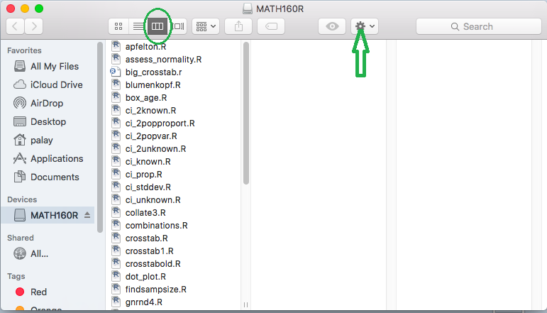
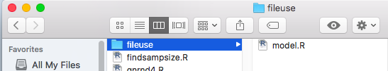
Please note that the USB drive that you were given was named "MATH160R" which is why you see that name on the icon shown in Figure 1. If you double click on that icon you will open a Finder window similar to that shown in Figure 2. Please note that on the computer I used to capture these images, Finder was set to display files in multiple panes, thus you see the icon circled in green in Figure 2 is in fact highlighted. If you do not have this icon highlighted then just click on it to change your display so that it looks like the one in Figure 2.

Figure 2

Each different example, project, or test that we do for this class will be done in a separate directory (folder) that is a sub-directory (sub-folder) of the MATH160R USB drive. Therefore, we need to create such a folder. To do that, click on the

icon in the top of the window shown in Figure 2. This will open the drop down box shown in Figure 3.

Figure 3

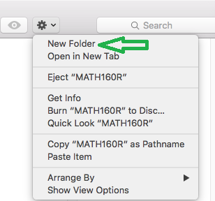
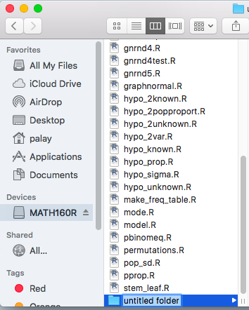
We want to create a new directory (folder) so we click on the New Folder option. The result is the creation of a new directory, called untitled folder on our MATH160R drive. This is shown in Figure 4.

Figure 4

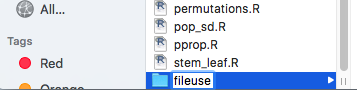
The default name, untitled folder is not helpful. We want to gve this a meaningful name. We will use the name fileuse. To do that we just type in that name as shown in Figure 5.

Figure 5

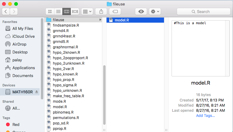
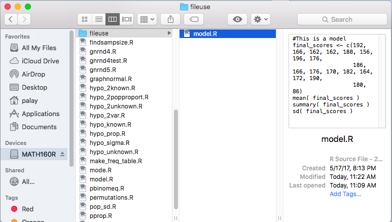
Now that we have the new folder fileuse we should note that it is a currently empty folder. We want to take a copy of the file model.R and place that copy into our new folder. We look up in the list of files that are on our MATH160r drive and we click on the model.R file in order to select it and have it highlighted, as shown in Figure 6.

Figure 6

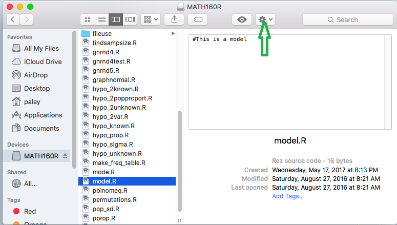
You might notice in Figure 6 that doing this selection also caused the contents of the model.R file to be shown in the right pane of that Figure 6 window. In fact, the model.R file contains exactly one line of text, namely, #This is a model. In effect this is a do nothing file and we just use it as a starting point for the work we really want to do.

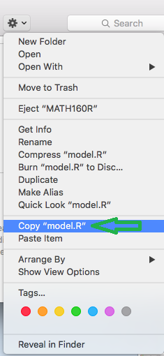
What we want is a copy of that file. To get this we return to click on the action icon,

, which then opens the drop down box shown in Figure 7. There we find and click on the action Copy "model.R".

Figure 7

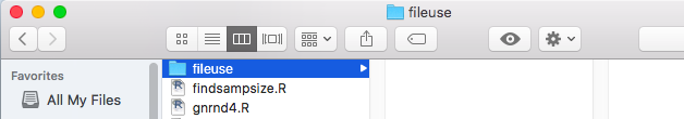
Once that is done we return to our list of files on the MATH160R drive and we highlight the directory (folder) that we just created, fileuse, as shown in Figure 8.

Figure 8

Now return to the actions. Click on the

icon to open the drop down box shown in Figure 9.

Figure 9

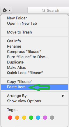
To paste the file that we copied, click on the Paste Item option in Figure 9. The result it just what we want, a copy of the model.R file is now in our fileuse sub-directory. We can see this in Figure 10.

Figure 10

At this point we want to use that file, model.R, the one in our sub-directory, fileuse, to open a RStudio session. We start that process by highlighting the file (click just once on the file), as shown in Figure 11.

Figure 11

Then, we will click on the actions icon,

, to open the drop down box shown in Figure 12. Once the box shows up, point to the Open With option. Doing so will open a secondary option box, shown in Figure 12 to the right of the option.

Figure 12

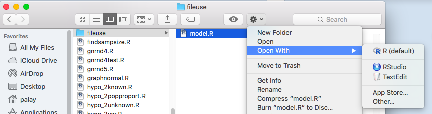
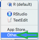
Figure 13 just shows that secondary box. Note that the default for running this file is R. However, this box also gives us the option of opening our model.R file with RStudio. We will not take either option! Instead we will choose the Other... option by clicking on it.

Figure 13

Doing so opens the list of applications installed on this computer as shown in Figure 14. We want to find RStudio in the list. We will have to scroll down to find it.

Figure 14

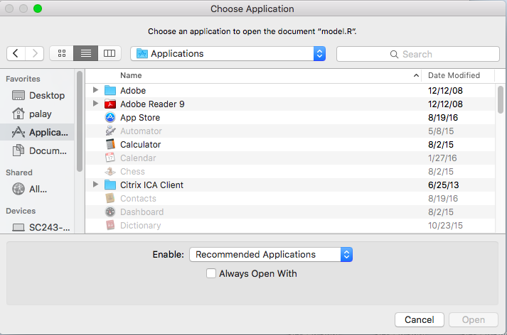
Figure 15 shows that we have scrolled down, found RStudio, and in fact we have clicked on it once to highlight it.

Figure 15

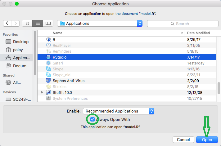
Before we leave Figure 15 we want to check the box, circled in green in Figure 15, for Always Open With. By checking this box and then clicking on the OPEN button we are telling this computer that files that end in .R are associated henceforth with RStudio. That means that in the future we can just double click on a file such as model.R to start a new session of RStudio.

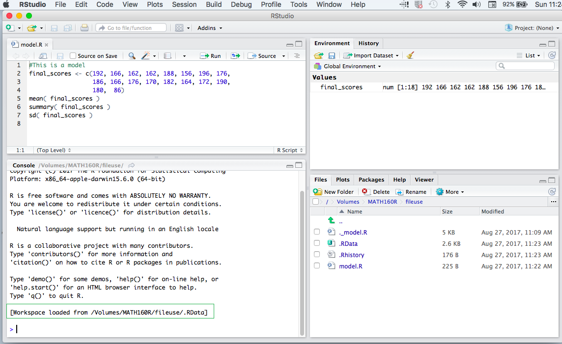
Once we click on the Open button a RStudio session starts. The opening screen for that is shown in Figure 16.

Figure 16

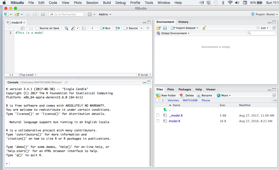
There are a number of things to note in Figure 16. First, we have 4 panes in this window. The upper left pane is an editor. In it we see the contents of our model.R file. Second, the lower left pane is the console pane. It holds an active R session. In Figure 16 we see the opening splash screen for R. Third, the upper right screen is the Environment pane. At the moment it is empty reflecting the fact that we are starting with nothing. And fourth, the lower right screen is showing the list of files in our current directory.

That last statement may be a bit of a shock. After all, when we started this, back in Figure 11, our directory, fileuse, held just one file, namely model.R. Figure 16 now tells us that there are two files in the directory, the new one called ._model.R. We will have to keep an eye on this.

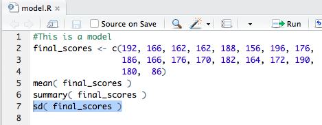
Our next step is to do a small example of using RStudio to do some work in R. The actual commands that we will type are:

final_scores <- c(192, 166, 162, 162, 188, 156, 196, 176,
                  186, 166, 176, 170, 182, 164, 172, 190,
                  180,  86)
mean( final_scores )
summary( final_scores )
sd( final_scores )

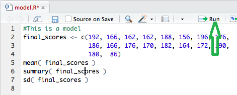
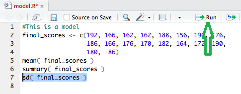
We will type them into the editor pane, thus being able to save them in our file model.R later. Figure 17 shows the status of the typing partway through the fourth line of text.

Figure 17

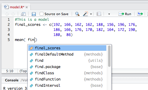
I stopped typing there to point out two things that you can notice as you type the commands. First RStudio automatically supplied the closing parenthesis. Second, as I started to type the name of the variable final_scores the line RStudio supplied a drop down box with possible completions. Once that was displayed, and given that the desired variable is highlighted in the box, in order to complete the name of the variable I just hit the Enter key producing Figure 18.

Figure 18

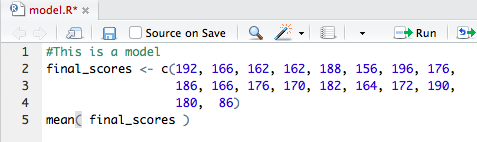
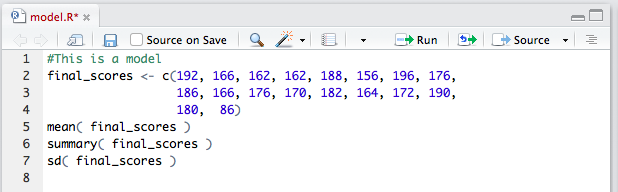
Figure 19 shows the completed text.

Figure 19

We will have R, remember that the R console display is shown in the lower left pane, perform the first two commands. To do this we start by highlighting the first 4 lines, as in Figure 20.

Figure 20

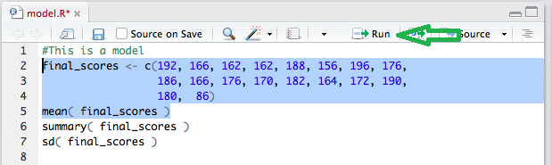
To submit those lines to R we click on the

at the top of the editor pane in Figure 20. We see the result, in the console pane in Figure 21.

Figure 21

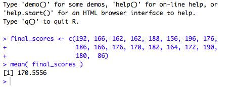
Our two commands have been accepted, without error, and they have been performed. Note that the commands appear in blue and the resulting output of the commands, in this case just the line

, appears in black. The [1] in that line just means that this is the first item of output from the command mean(), the 170.5556 is the value of the mean of all the values stored in final_scores.

There is another change that we need to examine. Look at the environment pane, shown in Figure 22.

Figure 22

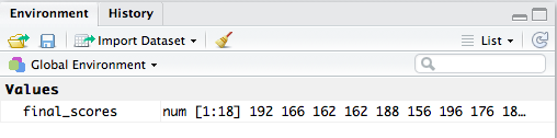
There we see that there is now a variable called final_scores that has been defined. (We did that when we had R perform the first three of the four lines we gave to it.) Furthermore, the environment pane goes on to tell us that this variable holds numeric values, that there are 18 such values, and the start of the listing of those values is

.

We return to the editor pane, shown in Figure 23.

Figure 23

Note that in Figure 23 we have placed the cursor in the

line. Before, back in Figure 20, we highlighted the lines that we wanted to submit to R. If we have just one line to submit, as we do here in Figure 23, we can get away with just having the cursor on the line and then clicking on the

icon. This will submit that one line which we will then see in the editor pane.

Figure 24

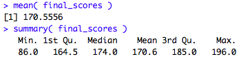
The result of the summary( final_scores ) command is shown in Figure 24. The six values give the minimum, first quartile, median, mean third quartile, and maximum values from those stored in final_scores.

We return to the editor pane and highlight the next command to run.

Figure 25

When we click on the Run icon in Figure 25 we get the Figure 26 output in Figure 26.

Figure 26

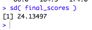
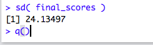
The sd() command produces the standard deviation of the values in final_scores, treating those values as if they represent a sample of a population. We see that the standard deviation is 24.13497.

That is all the work that we wish to do here. However, we want to observe a few other thisng. First, we return to look at the lower right pane, shown again in Figure 27. That information has not changed since we first saw it back in Figure 16.

Figure 27

Then return to the editor pane, shown in Figure 28.

Figure 28

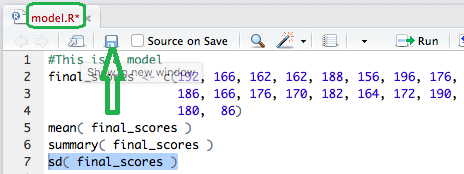
I have framed in green the name of the tab. Notice that the name is in red. This indicates that the contents of the editor have changed from what is in the file. In fact the name has been in red since Figure 16.

We click on the "floppy disk" icon in Figure 28 to take us to Figure 29.

Figure 29

Note that the name has changed back to being displayed in black. If we return our attention to the lower right pane, shown in Figure 30, we can see that the model.R file has had its file Modified attribute changed to reflect the version now saved.

Figure 30

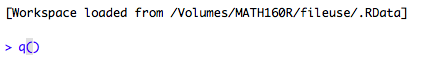
In order to actually quit our session we will go directly to the console pane, shown in Figure 31, and type the command q().

Figure 31

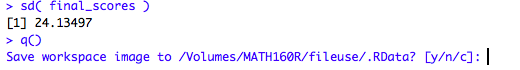
When we press the Enter key, R responds with the question shown in Figure 32. We do want to save the workspace so we will type y and press e Enter key to quit the session.

Figure 32

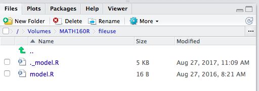
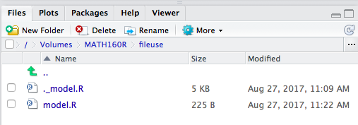
In Figure 33 we see again the Finder window that we left starting in Figure 11. However, now the contents of the file have been updated from our RStudio session. Also note the change in the timestamps at the lower right of the screen.

Figure 33

We do want to see the effect that our work back in in Figures 12 through 15 accomplished. Remember that RStudio is now the default program for files with the .R extension. Therefore, is we double click on the model.R file name in Figure 33 we immediately start the RStudio session shown in Figure 34.

Figure 34

There are a few things to note. First, the saved version of the model.R file is ready for us in the editor pane. Second, we have a new R session started in the console pane. Note the line boxed in green. The R session has loaded an environment from a file called /Volumes/MATH160R/fileuse/.RData. Third, the one variable that we had defined, namely, final_scores, has been restored to the environment pane. And fourth, the files pane now shows that there four files in our directory with .RData and .Rhistory being the new additions. [You might question the existence of the files other than model.R. After all, we just saw, in Figure 33, that Finder seems to believe that there is only one file in our sub-directory fileuse. The remaining files are "hidden" files. Finder, by default, does not display hidden files. Therefore, these files did not appear in Figure 33. The RStudio Files pane, however, will show all files.

That is enough for now. We return to the console pane and quit our session with our q() command.

Figure 35