Residuals

Return to Topics page
Another topic related to regression is residuals. Without using the name residuals we have been using the concept since we started working with regression. We start with some original data points, the observed values We generate a regression equation that has the smallest sum of the squares of the differences between the observed y values and the expected y values for all of the observed x values. The difference between an observed y value and its corresponding expected y value is the residual for the associated x-value. Consider the data in Table 1.
We can generate, display, and create the linear regression model for this data via the following commands:

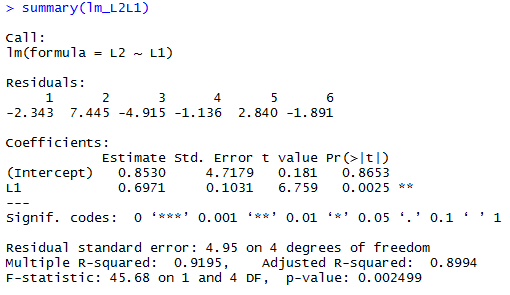
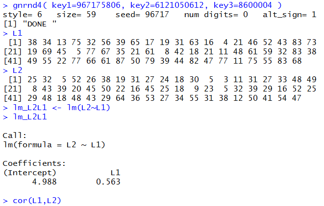
gnrnd4( key1=967170506, key2=6121050612, key3=8600004 )
L1
L2
lm_L2L1 <- lm(L2~L1)
lm_L2L1
cor(L1,L2)

These produce the console text in Figure 1.

Figure 1

We use the information in Figure 1 to form the regression equation, namely, y = 0.853 + 0.6971 * x.

We can even generate a plot of the observed points and the regression line via

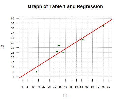
plot(L1,L2,xlim=c(0,80),xaxp=c(0,80,16),
     ylim=c(0,60),yaxp=c(0,60,12),
     main="Graph of Table 1 and Regression",
     las=1, cex.axis=0.7, pch=18, col="darkgreen")
abline(v=seq(0,80,5), col="darkgray", lty=3)
abline(h=seq(0,60,5), col="darkgray", lty=3)
abline(lm_L2L1, col="red", lwd=2)

That plot is shown in Figure 2.

Figure 2

We are looking for the residuals. To find the residuals we need to know, for each observed x value, both the associated observed y value and the associated expected y value. The commands

c_vals <- coefficients(lm_L2L1)
c_vals
y_vals <- c_vals[1]+c_vals[2]*L1
y_vals

first retrieve the intercept and coefficient of x from our model and store them in the variable c_vals. Then we display the values in c_vals, noting that they are the slightly longer versions of the values we saw in Figure 1. The statement y_vals<-c_vals[1]+c_vals[2]*L1 uses those values, along with the observed x values stored in L1, to implement the regression equation and, therefore, to compute all of the expected y values. Those are stored in the variable y_vals. The last line, y_vals, then displays the values. We use this just so that we can see those values.

Figure 3

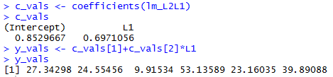
Those expected y values are the y coordinates for the associated x values of points on the regression line. We add the plot of these points to our graph via the command

points(L1,y_vals,pch=17,col="blue")

with the result shown in Figure 4.

Figure 4

On the graph we can represent the difference between the observed and expected y values by drawing a line segment between those points. The code

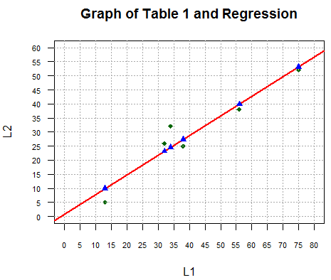
for(i in 1:length(L1))
  { lines(c(L1[i],L1[i]),c(L2[i],y_vals[i]),lwd=2)}

accomplishes this as we see in Figure 5.

Figure 5

Although the graphic representation is nice, we really want to get the numeric values for the residuals. The observed y values are in L2. The expected y values are in y_vals. The statements

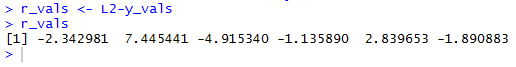
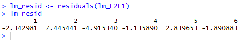
r_vals <- L2-y_vals
r_vals

find those differences, store the differences in r_vals and then display those residual values. The console result is shown in Figure 6. [When matching the values shown in Figure 6 with the line segments shown in Figure 5 remember that the values in Figure 6 are associated, in order, with the values in L1. Looking back at Table 1 we see that those values in L1 were not given in ascending order. Therefore, we need to check the x value in Table 1 to determine which of the line segments in Figure 5 matches which of the values shown in Figure 6.]

Figure 6

A most careful reader of these pages may recall that we actually saw a display of residuals in a much earlier page. There we used the summary() command to get more information about our linear model. We can use that command here, the summary(lm_L2L1) command, to see a great deal of information about the linear model that we stored in the variable lm_L2L1. Figure 7 shows the console output from that command.

Figure 7

Sure enough, there in Figure 7, are the residuals, though given with fewer decimal places.

Recall that we used the coefficients() function to pull the intercept and coefficient of x out of the linear model. In the same way, instead of computing the residuals as we did by finding the expected values (in Figure 3) and then the observed minus the expected values (in Figure 7), we could have just used the function residuals() to extract the values from the linear model. The command would be lm_resid<-residuals(lm_L2L1) as shown in Figure 8.

Figure 8

The values shown in Figure 8 match the values we worked so hard to produce earlier.

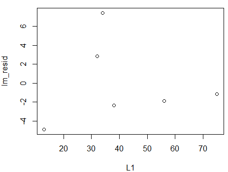
Residuals are important because we want to be sure that there is no apparent pattern to them. That is, if we plot the residuals (by matching the residual value to its associated x value), then the plotted points shown seem randomly placed on the graph. For our problem a quick and simple statement such as plot(L1,lm_resid) will produce such a graph, in this case the gaph in Figure 9.

Figure 9

Table 1 only had 6 values in it. With so few values it is hard to see or even not see a pattern in the residual plot. Perhaps it would be better to look at a slightly larger problem.

Table 2 provides the data for a new problem.
This example has 59 pairs of values. However, the analysis process is the same. As before, we use

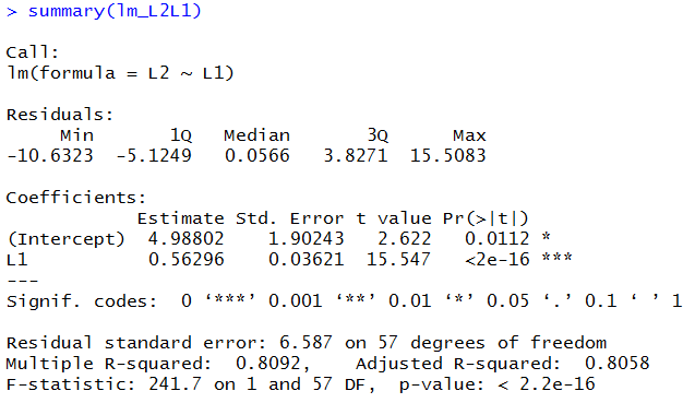
gnrnd4( key1=967175806, key2=6121050612, key3=8600004 )
L1
L2
lm_L2L1 <- lm(L2~L1)
lm_L2L1
cor(L1,L2)

to generate and display (just for verification) the data, as well as to create and display a new linear model. Console output is shown in Figure 10.

Figure 10

The commands

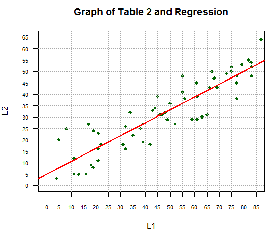
plot(L1,L2,xlim=c(0,85),xaxp=c(0,85,17),
     ylim=c(0,65),yaxp=c(0,65,13),
     main="Graph of Table 2 and Regression",
     las=1, cex.axis=0.7, pch=18, col="darkgreen")
abline(v=seq(0,85,5), col="darkgray", lty=3)
abline(h=seq(0,65,5), col="darkgray", lty=3)
abline(lm_L2L1, col="red", lwd=2)

produce a graph, as shown in Figure 11.

Figure 11

Although we learned above that to just find the residuals we could jump down to the commands following Figure 15, here we will walk through our process just to illustrate what R has already done for us.

We generate the expected y values via

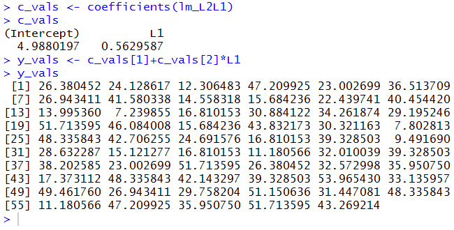
c_vals <- coefficients(lm_L2L1)
c_vals
y_vals <- c_vals[1]+c_vals[2]*L1
y_vals

with the console output in Figure 12.

Figure 12

We graph the expected points and draw the line segments via

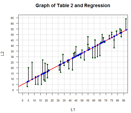
points(L1,y_vals,pch=17,col="blue")
for(i in 1:length(L1))
{ lines(c(L1[i],L1[i]),c(L2[i],y_vals[i]),lwd=2)}

changing the graph to that in Figure 13.

Figure 13

We compute and display the residuals via

r_vals <- L2-y_vals
r_vals

as shown in Figure 14.

Figure 14

Then, just so that we can see the values we use the summary(lm_L2L1) command to produce the more detailed display of the values in our linear model. That display is shown in Figure 15.

Figure 15

Note that there is a subtle change to the format of the output in Figure 15 compared to the format that we saw back in Figure 7. In the earlier display, R actually gave us the 6 residual values. Here, in Figure 15, rather than display all 59 values, R shows us a summary of those values, namely the Min, 1Q, Median, 3Q, and Max values. Note that our linear model still has the residual values in it, but the workings of the summary() command have changed to show these 5 summary values rather than to display all of the individual residual values.

We use the commands

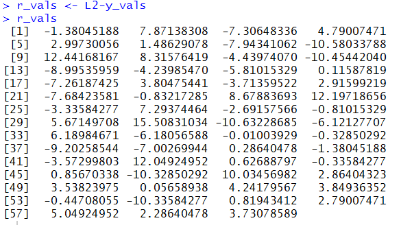
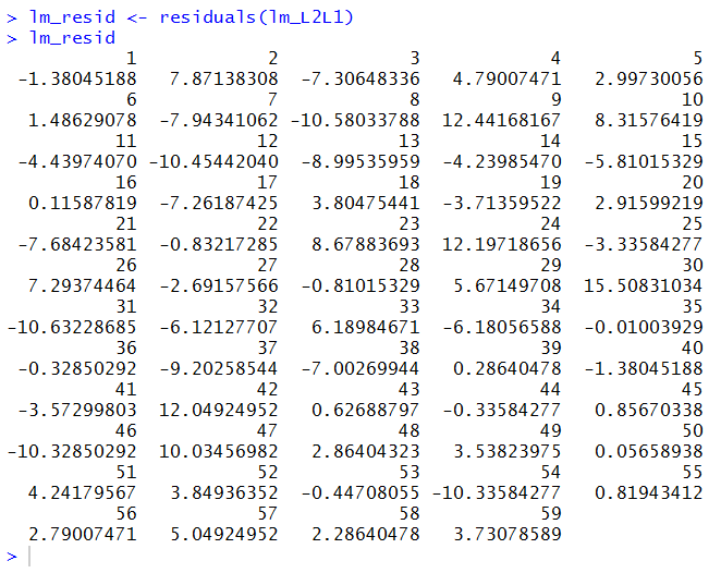
lm_resid <- residuals(lm_L2L1)
lm_resid

to retrieve the residual values from our model and to display those values, as shown in Figure 16.

Figure 16

The display in Figure 16 takes up a bit more room than did our earleir display, in Figure 14, of the r_vals that we had computed. This longer display is just a change in formatting style where the Figure 16 version also gives the position number of the residual values.

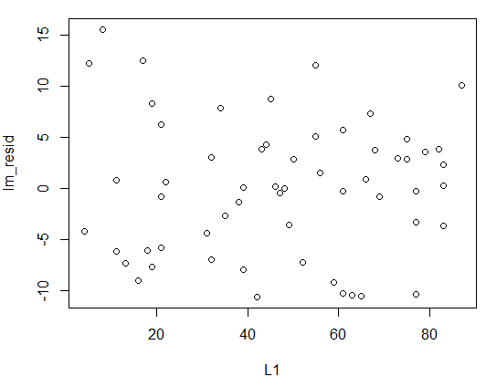
Finally, we use the command plot(L1,lm_resid) to plot the residuals so that we can see that there is no real pattern to them. The plot appears in Figure 17.

Figure 17