Independence and Chi-Squared test for independence

Independence and χ² test for independence

Return to Topics page
Consider the situation where we have two ways to categorize a population. An example would be to group people by age and also to group them by their preference for certain ethnic foods. A person will fall into one age category and one preference for ethnic foods. We can take a sample of the population and count the number of people in each combination of categories. This sample would be represented by the following table.
The question that we want to investigate is "Does there exist a relationship between a person's age and their preference for a particular type of ethnic food?" In general, and we will further define this below, such a "relationship" is just a mathematical statement of fact; it is not a claim of causality. If knowing a person's age changes our expectations on their preference for a type of ethnic food, then there is a relationship between the two concepts. The same is true if knowing a person's preference for a type of ethnic food changes our expectations about the person's age.

To see this in action we will first examine a case where knowing one feature is absolutely no help in improving our guess at the other. The data in Table 3 represents such a perfect case.

For all 630 people in Table 3, 1/3 of them are under 11, 1/2 of them are between 11 and 18 inclusive, and 1/6 of them are over 18. Those same relations hold within each group of people for each type of ethnic food. Thus, for the 210 people who prefer Indian cuisine 1/3 are under 11, 1/2 are between 11 and 18 inclusive, and 1/6 are over 18. Therefore, knowing that a person prefers Italian cuisine does not change your expectations about the age of the person.

In a similar manner, for all 630 people in Table 3, 1/15 of them prefer Mexican cuisine. The same is true across all age groups. Of the 315 people who are between 11 and 18 years old, exactly 1/15 of them prefer Mexican cuisine. Of the 105 people who are over 18, exactly 1/15 of them prefer Mexican food.

Compare the situation shown in Table 3 to the one shown in Table 4.
For the 630 people in Table 4 approximately 29.36% of them are under 11. However, for the 60 people who prefer Chinese food, 25% of them are under 11. For the 630 people in Table 4 approximately 30.16% of them are between 11 and 18. However, for the 60 people who prefer Chinese food, 36.67% of them are between 11 and 18. For the 630 people in Table 4 approximately 40.48% of them are over 18. However, for the 60 people who prefer Chinese food, 38.33% of them are over 18. Thus, if we know that a person prefers Chinese food then our expectations of their age are quite different.

In a similar manner, for all 603 people, approximately 18.10% prefer Mexican food. However, knowing that a person is over 18 changes our expectations because for that age group approximately 25.26% of the 114 people are over 18.

Independence: If knowing one factor for a population does not change the distribution of the other factor of the population then the two factors are said to be independent. Notice that this is a purely mathematical statement. It just talks about the distribution of a factor within a population and then within a subgroup (determined by a different factor) of the population.

There are computed values that can help us see such independence. For example, Table 5 expresses the relationships of Table 3 but as percentages of the row totals. That is, we take every value in Table 3 and divide it by the value in the final column of the same row.

Notice that knowing an age group does not change the percent associated with each food type.

We could do the same thing for Table 4 and show that in Table 6.

Now we see, in Table 6, that the distribution across columns changes depending upon which row we are in. That is why, for Table 4, knowing an age group changes our expectation for the food preference.

There is nothing special about using row totals as we did in Table 5 and Table 6. We could just as easily generate a companion table that shows the percent of the column totals, i.e., the percent of the number in the final row. Table 7 shows the percent of the column totals for the data in Table 3.

As we saw above, because Table 3 represents independence between the factors, each of the column distributions is the same as that of the final column.

We get quite different results when we look at the percent of column totals in Table 4 as is shown in Table 8.

In Table 8 we see clear evidence of the different expectations that we would have for the food age of a person if we knew their food preference.

Expected Value: In Table 2, Table 3, and Table 4 we have seen three different distributions for the two factors, age and food preference. Each of those tables give the row totals and the column totals. If the distribution is independent then we expect that

Each data row of the table will have the same distribution as that of the final row, the column totals.
Each data column of the table will have the same distribution as that of the final column, the row totals.

This will happen if and only if each data cell has a value that is equal to the distribution for that row times the distribution for that column times the total number of items in the table. Such a value is called the expected value. The row distribution for Table 4 was shown as the final column in Table 8. It was 29.37%, 40.48%, and 30.16%. The column distribution for Table 4 was shown as the final row in Table 6. It was 9.52%, 18.10%, 14.76%, 23.81%, and 33.81%. Thus, the expected value in Table 4, which has 630 individuals, for the number of people who are under 11 and who prefer Chinese food is (under 11 row percent)(prefer Chinese food column percent)(630)
(29.37%)(9.52%)(630)
17.615 The expected value for the number of people who are between 11 and 18 and who prefer Italian food is ("11 to 18" row percent)(prefer Italian food column percent)(630)
(40.48%)(14.76%)(630)
37.643 We need to compute all 15 such expected values. The result would be Table 9.

The computation of the values in Table 9. need not be as complicated as indicated above. In general, the rule above is

value in the cell in row I column J	=	Percent of row I total	*	Percent of column J total	*	Grand Total
but that is the same as
value in the cell in row I column J	=	row I total Grand Total	*	column J total Grand Total	*	Grand Total
but that is the same as
value in the cell in row I column J	=	row I total * column J total Grand Total

Table 9 showed the expected values generated from the row and column totals back in Table 4. Remember that Table 4 was presented as a relation that was definitely not independent. Therefore, it should not be a surprise to find that the expected values in Table 9, the 15 data values, are different from the observed values in Table 4.

Recall that Table 3 was presented as a perfectly independent relation. If we do the same calculation on Table 3, multiplying row totals by column totals and dividing by the grand total, to get expected values, then we really should expect to get exactly the same values that we observed in Table 3. Here is a restatement of Table 3.

Then, Table 10 is a statement of the expected values generated from the row and column totals of Table 3.

Although it may "look like" we have just copied the values from Table 3 to Table 10, that is not the case. Table 10 is the result of the same computation pattern used to generate Table 9 from Table 4. In this case, however, because Table 3 represents a perfectly independent relation, there is no difference between the observed and the expected values.

What about our original data, the relation shown in Table 1 and then shown again, with row and column totals, in Table 2? First, we will restate Table 2.

Then we produce Table 11 to show the expected values derived from the row and column totals of Table 2.

Clearly, the observed values of Table 2 are different than the expected values of Table 11. That means that for the 630 people involved, the relationship shown in Table 2 is not independent.

Just thinking about the requirement for independence it would be quite strange to find a relationship that is independent. Move just one person from one category to another and the perfect independence of the relationship in Table 3 would be destroyed. Not by much, but we would not have that perfect fit any longer. Fortunately, we are usually not concerned with the difficulty in having a perfect fit.

Our usual case is that we have a large population with two "factors" or "categories" as we have seen above and we have a sample of that population. For example, our population might be the residents of Manhattan. Our sample might be the 630 people represented in any of Tables 2, 3, or 4. Our question is "For the population, are age group and preference for food type independent?" Now we are in the familiar territory of making a judgement about a population based on a sample.

Our null hypothesis is H₀: the two are independent and our alternative hypothesis is H₁: the two are not independent. We decide that we want to test H₀ at the 0.05 level of significance. We take a sample and based on that sample, assuming H₀ is true, how strange would it be to get a sample such as the one we have.

If our sample was the 630 people shown in Table 3, the table with a perfect fit, where the expected values, shown in Table 10, are identical to the observed values, then we have no evidence to reject H₀. On the other hand, if our sample was the 630 people shown in Table 4, the table where the expected values, shown in Table 9, are far from the observed values, then we might have enough evidence to reject H₀. To do this we need to have a sample statistic, a value that we can compute from the sample, and a distribution of that statistic. Fortunately for this situation we have both.

The sample statistic will be the sum of the quotient of the squared differences between each of the observed values and their corresponding expected values divided by the expected value. Let us start with a restatement of Table 4 and Table 9.

Then we can compute the differences, the observed - expected values and get Table 12.;

Next we can square the differences and get Table 13.;

Then we can divide each square of the differences by the expected value to get Table 14.;
This is a measure of how far the expected values are from the observed values. If this number is large enough then we will have sufficient evidence to reject the null hypothesis.

How large does this sum of the quotients of the squared differences divided by the expected values have to be? In the case that all of the expected values are greater than 5, that sum will be distributed as a χ² distribution with the number of degrees of freedom equal to the product of the one less than number of rows times one less than the number of columns.

If it turns out that one or more of the expected values in the cells of the table are 5 or less then we need to stop the interpretation. Increasing the overall sample size may alleviate such a deficiency. In this example all of the expected values, shown back in Table 9 are greater than 5. Therefore, we can continue with this interpretation.

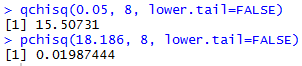
In our example that means that we will have (3-1)*(5-1) = 2*4 = 8 degrees of freedom. The χ² value with 8 degrees of freedom that has 5% of the area to the right of it is about 15.507. This is our critical value. Our sample statistic of 18.186 is more extreme than this so we say that we have sufficient evidence to reject H₀ at the 0.05 level of significance. Were we to ask for the attained significance we would be asking for the area under the χ² curve with 8 degrees of freedom that is to the right of 18.186. That attained significance is 0.01987, a value less than our 0.05 significance level, so we reject H₀ at the 0,05 level.

The R statements needed to find our critical value and then our attained significance value are

qchisq(0.05, 8, lower.tail=FALSE)
pchisq(18.186, 8, lower.tail=FALSE)

respectively. The console view of those statements is shown in Figure 1.

Figure 1

All of this means that if our random sample of 630 people had the distribution of responses shown in Table 4 then we would have sufficient evidence to reject H₀. I must confess that the values in Table 4 were adjusted to achieve just that result. However, the values in Table 1, and repeated in Table 2 were not adjusted. Let us go through the same process with those values. We will restate the values in Table 2.

Then we produce the table of expected values. We did this before in Table 11 so we can restate it here.

Then we can compute the differences, the observed - expected values and get Table 15.;

Next, we can square the differences and get Table 16.;

Then we can divide each square of the differences by the expected value to get Table 17.;

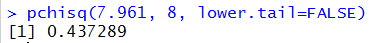
The number of rows and column has not changed from the earlier example. Therefore, we still have 8 degrees of freedom and the χ² value with 5% of the area to the right of that value remains 15.507 so that is our critical value. The sample statistic that we just computed was 7.961, a value that is not more extreme than the critical value. Therefore, we say that we do not have sufficient evidence to reject the null hypothesis.

Although the command to find the critical value remains unchanged from Figure 1, the command to find the attained significance needs to change to

pchisq(7.961, 8, lower.tail=FALSE)

The console version of that statement is given in Figure 2.

Figure 2

In order to reject the null hypothesis we need an attained significance that is less than our pre-set significance level. Since 0.437 is not less than 0.05 we do not have sufficient evidence to reject the null hypothesis.

This is a good place to emphasize our conclusion. To do the test we assume that H₀ is true, that for the population the two factors are independent. Now the truth is that if we interviewed everyone in the population and formed the table of responses there is little chance that the numbers would fall into that perfect independence illustrated by Table 3. However, we are not going to dwell on that. Instead, we assume that the two are independent and we take a sample. We generate our sample statistic from that data. If the value of that sample statistic is larger than our critical value, then we can justify rejecting the null hypothesis. Otherwise we cannot justify rejecting it. Alternatively, if the attained significance of that sample statistic is less than the level of significance that we had agreed to for the test, then we have evidence to reject the null hypothesis. Again, otherwise, we do not have sufficient evidence to reject the null hypothesis.

We have seen a process for generating our sample statistic, namely;

get the row and column totals
generate the expected values
find the difference between the observed and the expected values
find the square of those differences
find the quotient of the square of the differences divided by the expected values
get the sum of all of those quotients

This web page demonstrated each of those steps for the two examples that we have considered. Although you can follow along on the web page, and although you could do the work by hand, we have not seen any way to do these computations in R. We will now fill that void.

First, consider the commands. Note that extensive comments have been added so that you can follow along in the sequence of commands.

source("../gnrnd4.R")

gnrnd4( key1=342314108, key2=8756454753 )
# the gnrnd4 produced a matrix to hold
# the observed values.  We need to get
# the structure of that matrix
base_dim <- dim(matrix_A)
num_row<-base_dim[1]
num_col<-base_dim[2]
# while we are at it, rather than 
# mess with the original matrix we will 
# make a copy of it
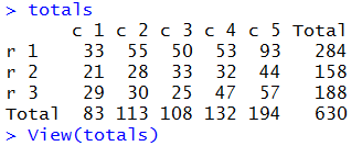
totals <- matrix_A
# then we can get all of the row sums
rs <- rowSums( totals )
# and append them, as a final column,
# to our matrix totals
totals <-cbind(totals,rs)

# next we can get the column sums,
# including the sum of the column we 
# just added, the one holding the row sums
cs <- colSums( totals )
# and we can append that to the 
# bottom of the totals matrix
totals <- rbind(totals,cs)
# Now, just to "pretty up" the structure we
# will give appropriate names to the
# rows and columns

col_names <- "c 1"
for( i in 2:num_col)
{ col_names <- c(col_names, paste("c",i))}
col_names<-c(col_names,"Total")

row_names <- "r 1"
for (i in 2:num_row)
{ row_names <- c(row_names, paste("r",i))}
row_names <- c(row_names,"Total")

rownames(totals)<-row_names
colnames(totals)<-col_names
# Finally look at the matrix, here and
# with the fancy image.
totals
View(totals)

The real output from these commands is from the last two lines. The console output is shown in Figure 3.

Figure 3

The fancy table produced within RStudio is shown in Figure 4.

Figure 4

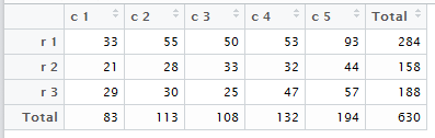
Both of these are the R version of Table 2. Now we need to generate the expected values. The following commands do that.


# Create a matrix with the expected values.
# The column totals are held in cs
# and the row totals are held in rs

# get the grand total, store it in t
t <- cs[num_col+1]

expected <-matrix_A
for ( i in 1:num_row)
{  rowtot <- rs[i]
   
   for ( j in 1:num_col)
   { expected[i,j] <- rowtot*cs[j]/t}

}
# take a look at this matrix
expected
View( expected )

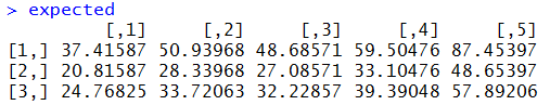
Again, the real output from the final two lines, the first of which produces Figure 5 in the console.

Figure 5

The last command produces the fancy table shown in Figure 6.

Figure 6

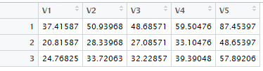
Figure 5 and Figure 6 hold the R equivalent of Table 11.

The next step is to find the observed - expected values. Consider the statements

# to get the observed - expected
# we can use the two matrices. Note that 
# we cannot use totals here because it is
# now a different size, having added the 
# row and column totals.
diff <- matrix_A - expected
diff
View( diff )

The second to last statement produces Figure 7.

Figure 7

The final statement produces Figure 8.

Figure 8

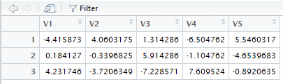
Figure 7 and Figure 8 correspond to Table 15.

The following commands generate and display the square of the differences.

# get the square of the differences
diff_sqr <- diff * diff
diff_sqr
View( diff_sqr )

Figure 9 shows the console output.

Figure 9

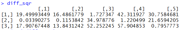
Figure 10 shows the "pretty" output.

Figure 10

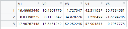
The values shown in Figure 9 and Figure 10 correspond to the values in Table 16.

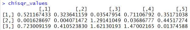
The last version of the table that we need holds the quotient of the squared deviations and the expected values. The commands to produce and view that table are:

# now get the quotient of the squared
# differences and the expected value
chisqr_values <- diff_sqr/expected
chisqr_values
View( chisqr_values )

That produces the output in Figure 11.

Figure 11

It also produces the view shown in Figure 12.

Figure 12

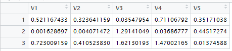
Figure 11 and Figure 12 correspond to Table 17.

Now we need to find the sum of the values in Figure 11, along with the degrees of freedom that we want to use, and then the attained significance for that sum using that number of degrees of freedom. In R we can do this with the statements

# Finally we need to get the sum of the
# values in that final table
x <- sum(chisqr_values)
x
# then find the attained significance 
# of that sum
use_df <- (num_row-1)*(num_col-1)
use_df
attained <- pchisq( x, use_df,
                    lower.tail=FALSE)
attained

The console view of this is shown in Figure 13.

Figure 13

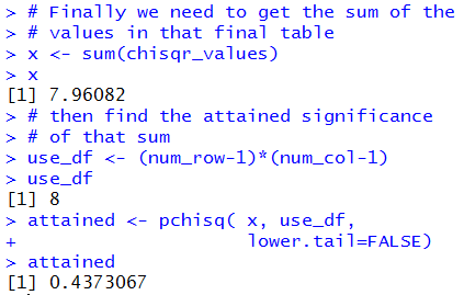
The information shown in Figure 13 is the same as the information that we saw in Figure 2.

The commands above, following the use of the gnrnd4() command, could be used to analyze any similar problem. To help in doing this, the entire sequence of commands appears at the end of this page so that you can highlight it, copy it, and paste it into your R session to run it for a new problem. However, it makes sense to just capture all of this in a function. While we are constructing such a function we can add a few features to it. This will include

A new table that gives the percent of each item compared to the row total. This is called a row percent.
A new table that gives the percent of each item compared to the column total. This is called a column percent
A new table that gives the percent of each item compared to the overall total. This is called the total percent.
Changing the workings of the function so that it produces all of these tables in the general environment. This means that although the tables are produced in the function they are visible and available in the regular environment.
Producing output that includes the final sum, called the chi-squared value, the degrees of freedom, and the attained significance.

Such a function is available at the crosstab.R link. Assuming that this function has been downloaded to your parent directory, the following two commands load and execute the function for the original data in matrix_A.

source("../crosstab.R")
crosstab( matrix_A)

The result is shown in Figure 14.

Figure 14

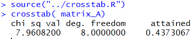
The function effectively replaces all of the work that we did above it. To demonstrate this we can clear out all of the old work and start over, first generating the the data again and then using the crosstab() function to perform everything. The commands to do this would be:

## clear out everything and start over,
## but just use the function.
rm( list=ls() )
source("../gnrnd4.R")
gnrnd4( key1=342314108, key2=8756454753 )
source("../crosstab.R")
crosstab( matrix_A)

The console view of those commands is shown in Figure 15.

Figure 15

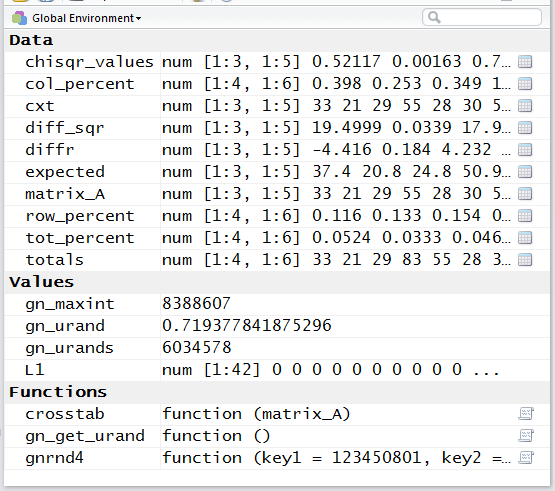
The resulting Environment pane in the RStudio session is shown in Figure 16.

Figure 16

The Editor pane of the RStudio session appears as Figure 17.

Figure 17

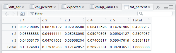
In Figure 17 we see the newly created total percent table. Each cell in that table gives the value of the corresponding original data value divided by the total number of entries in the original data.

Notice, in Figure 17, that there are many other tabs to allow us to get to other Views of the many tables that the function created. We can use the "back arrow" shown in Figure 17 on the left side of the screen and just below the list of tabs to navigate to other tabs. For example, we could move back to the totals tab as shown in Figure 18.

Figure 18

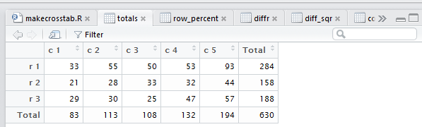
The totals table is the original data with the row and column totals appended to it.

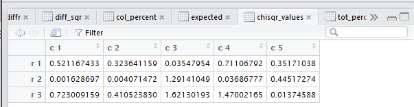
Now we can navigate, using the right arrow shown in Figure 18, to the chisqr_values tab. This is shown in Figure 19.

Figure 19

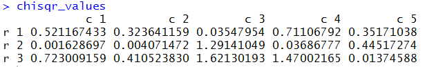
If, on the other hand, we want to see those values in the console output, because the chisqr_values variable is in the current environment (see Figure 16), we just need to use the variable name, chisqr_values in the console window and that table will be displayed there, as in Figure 20.

Figure 20

It is only fair to point out that the crosstab() function provided here is just a simple, and actually not very elegant, solution to perform this task. There are many other, more elegant and sophisticated solutions that are available in various packages within the R community. This one was written and provided because it shows all of the steps in the process.

Finally, if all you want to do is to perform a χ²-test for independence of the data in matrix_A this can be done in R without our new function by using the built-in function chisq.test() as

chisq.test(matrix_A)

which produces the output shown in Figure 21.

Figure 21

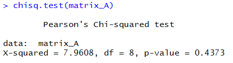
This does all of the work for us, but it does not show the intermediate steps.

Here is a listing of all the commands that were used to create this page.

qchisq(0.05, 8, lower.tail=FALSE)
pchisq(18.186, 8, lower.tail=FALSE)
pchisq(7.961, 8, lower.tail=FALSE)

source("../gnrnd4.R")

gnrnd4( key1=342314108, key2=8756454753 )
# the gnrnd4 produced a matrix to hold
# the observed values.  We need to get
# the structure of that matrix
base_dim <- dim(matrix_A)
num_row<-base_dim[1]
num_col<-base_dim[2]
# while we are at it, rather than 
# mess with the original matrix we will 
# make a copy of it
totals <- matrix_A
# then we can get all of the row sums
rs <- rowSums( totals )
# and append them, as a final column,
# to our matrix totals
totals <-cbind(totals,rs)

# next we can get the column sums,
# including the sum of the column we 
# just added, the one holding the row sums
cs <- colSums( totals )
# and we can append that to the 
# bottom of the totals matrix
totals <- rbind(totals,cs)
# Now, just to "pretty up" the structure we
# will give appropriate names to the
# rows and columns

col_names <- "c 1"
for( i in 2:num_col)
{ col_names <- c(col_names, paste("c",i))}
col_names<-c(col_names,"Total")

row_names <- "r 1"
for (i in 2:num_row)
{ row_names <- c(row_names, paste("r",i))}
row_names <- c(row_names,"Total")

rownames(totals)<-row_names
colnames(totals)<-col_names
# Finally look at the matrix, here and
# with the fancy image.
totals
View(totals)

# Create a matrix with the expected values.
# The column totals are held in cs
# and the row totals are held in rs

# get the grand total, store it in t
t <- cs[num_col+1]

expected <-matrix_A
for ( i in 1:num_row)
{  rowtot <- rs[i]
   
   for ( j in 1:num_col)
   { expected[i,j] <- rowtot*cs[j]/t}

}
# take a look at this matrix
expected
View( expected )

# to get the observed - expected
# we can use the two matrices. Note that 
# we cannot use totals here because it is
# now a different size, having added the 
# row and column totals.
diff <- matrix_A - expected
diff
View( diff )

# get the square of the differences
diff_sqr <- diff * diff
diff_sqr
View( diff_sqr )

# now get the quotient of the squared
# differences and the expected value
chisqr_values <- diff_sqr/expected
chisqr_values
View( chisqr_values )

# Finally we need to get the sum of the
# values in that final table
x <- sum(chisqr_values)
x
# then find the attained significance 
# of that sum
use_df <- (num_row-1)*(num_col-1)
use_df
attained <- pchisq( x, use_df,
                    lower.tail=FALSE)
attained

source("../crosstab.R")
crosstab( matrix_A)

## clear out everything and start over, 
## but just use the function.
rm( list=ls() )
source("../gnrnd4.R")
gnrnd4( key1=342314108, key2=8756454753 )
source("../crosstab.R")
crosstab( matrix_A)

chisq.test(matrix_A)