Hypothesis test for Population Mean, based on the sample mean, sigma unknown

Hypothesis test for Population Mean, based on the sample mean, σ unknown

Return to Topics page
The situation is:

We have a hypothesis about the "true" value of a population mean. That is, someone (perhaps us) claims that H₀: μ = a, for some value a.
Not unexpectedly, we do not know the population standard deviation, σ.
We will consider an alternative hypothesis which is one of the following
- H₁: μ > a,
- H₁: μ < a, or
- H₁: μ ≠ a.
We want to test H₀ against H₁.
We have already determined the level of significance that we will use for this test. The level of significance, α, is the chance that we are willing to take that we will make a Type I error, that is, that we will reject H₀ when, in fact, it is true.

Immediately, we recognize that samples of size n drawn from this population with have a distribution of the sample mean that is a Student's t with n-1 degrees of freedom. At this point we proceed via the critical value approach or by the attained significance approach. These are just different ways to create a situation where we can finally make a decision. The critical value approach tended to be used more often when everyone needed to use the tables. The attained significance approach is more commonly used now that we have calculators and computers to do the computations. Of course either approach can be done with tables, calculators, or computers. Either approach gives the same final result.

Critical Value Approach

We determine a sample size n. This will set the number of degrees of freedom as we use the Student's t distribution.
We find the t-score that corresponds to having the level of significance area more extreme than that t-score, remembering that if we are looking at being either too low or too high then we need half the area in both extremes.
Then, we take a random sample of size n from the population.
We compute the sample mean, and the sample standard deviation, s
Compute s_x = s / sqrt(n) and use that value to compute (t)(s_x).
Set the critical value (or values in the case of a two-sided test) such that it (they) mark the value(s) that is (are) that distance, (t)(s_x), away from the mean given by H₀: μ = a.
If the sample mean, , is more extreme than the critical value(s) then we say that "we reject H₀ in favor of the alternate H₁". If the sample mean is not more extreme than the critical value(s) then we say "we have insufficient evidence to reject H₀".

Attained significance Approach

Then, we take a random sample of size n from the population.
We compute the sample mean, and the sample standard deviation, s.
Assuming that H₀ is true, we compute the probability of getting the value or a value more extreme than the sample mean. We can do this using the fact that the distribution of sample means for samples of size n is a Student's t distribution with n-1 degrees of freedom with mean=μ and standard deviation=s/sqrt(n).
If the resulting probability is smaller than or equal to the predetermined level of significance then we say that "we reject H₀ in favor of the alternate H₁". If the resulting probability is not less than the predetermined level of significance then we say "we have insufficient evidence to reject H₀".

We will work our way through an example to see this. Assume that we have a population of values and that we do not know the standard deviation of those values in the population. I claim that the mean of the population, μ is equal to 134. You do not believe me. You think the mean of the population is not equal to 134. Notice that you are not saying what the true mean is, just that it is not 134.

It is hard for you to tell me that I am wrong, so you decide that you will take a sample of the population, compute the sample mean and the sample standard deviation. Then you will see just how strange that sample mean is, especially knowing the sample standard deviation. You happen to know that sample means from samples of size 36 from a population will follow a Student's t distribution with 35 degrees of freedom and will have the standard deviation of the sample mean, s_x, be equal to s / √36. Until we take a sample we will not know the value s and, therefore, we will not be able to compute s_x. However, if were to turn out that s_x is around 2.5 then clearly if you get a sample mean of 200, you are going to tell me that I am completely wrong. The value 200 is over 25 standard deviations above the value 134, the value we would expect to get if the true mean is 134. Random sampling is just not going to produce that kind of rare event. Well, it could happen, but the odds against it are so great you just say it is too unlikely to happen and reject my hypothesis.

On the other hand, if the sample mean turns out to be 134.7 then you would never think that getting such a sample mean would justify your claim that I am wrong. You have seen many examples where the sample mean changes with each sample and where the value of the sample mean is often more than one standard deviation away from the true population mean. In fact, you recall that for 35 degrees of freedom about 67.6% of the values in a Student's t distributed population are within 1 standard deviation of the mean. That means that about 32.4% of the values are more than 1 standard deviation away from the mean. We expect that nearly 1/3 of the time a sample of 36 items taken from our population (where for this part of the discussion we are assuming that sample yields s_x=2.5) will have values for the sample maean that are more than 2.5 above or below the true mean. If the true mean is 134 then getting a 36-item sample mean of that population that is 0.7 or more above or below 134 should happen really often (in fact, nearly 49% of the time).

If we are using the critical value approach, the question becomes, at what point is the sample mean far enough away from the supposed 134 for you to say that getting such a sample mean is just too unlikely; for you to risk claiming that my 134 value cannot be right because if it were then it is just too unlikely that you would get a 36-item random sample with such an extremely different sample mean. You answer that question by using the level of significance that you specify. If you are only willing to make a Type I error 1% of the time, then you want to find a value for the sample mean that is so extreme that only 1% of the Student's t distribution of 36-item sample means will be that or more extremely different from my hypothesis value of 134.

For this example, an extreme value can be too high or too low. You need to split the 1% error that you are willing to make between these two options. You know (from the tables, a calculator, or qt() ) that less than 0.5% (0.005 square units) of the area under the Student's t curve for 35 degrees of freedom is less than the t-score = -2.724 [and, correspondingly, less than 0.5% of the area under the standard normal curve is greater than 2.724]. Therefore, you know that being more than 2.724 standard deviations above or below the true population mean will happen less than 1% of the time.

We can do all of that computation, but we still do not know the value of s_x because we have yet to actually take a sample.

Now you take your sample. The values of that sample are shown in Table 1.

The computations that we did above are pretty straight forward. We could do them based on the values stored in L1, in R using:

n<-length(L1)
n
t <- qt(0.005,n-1,lower.tail=FALSE)
t
samp_sd <- sd(L1)
samp_sd
s_x <- samp_sd / sqrt(n)
s_x
to_be_extreme <- t*s_x
to_be_extreme
crit_low <- 134 - to_be_extreme
crit_high <- 134 + to_be_extreme
crit_low
crit_high
samp_mean <- mean(L1)
samp_mean

Unfortunately, I cannot show the R computation for the mean of the values in Table 1 above because the reproductions of the R screens are static whereas the values in the table are dynamic, they change whenever the page is refreshed. It should be enough, at this point in the course, to say that if you use the gnrnd4() command as given above, then the data will be in L1 and the commands will produce the values we just computed above.

I did, however, capture two earlier random tables, and I can reporduce them here. The first is shown in Table 1a.
Figure 1a shows generating the table and making those computations in R.

Figure 1a

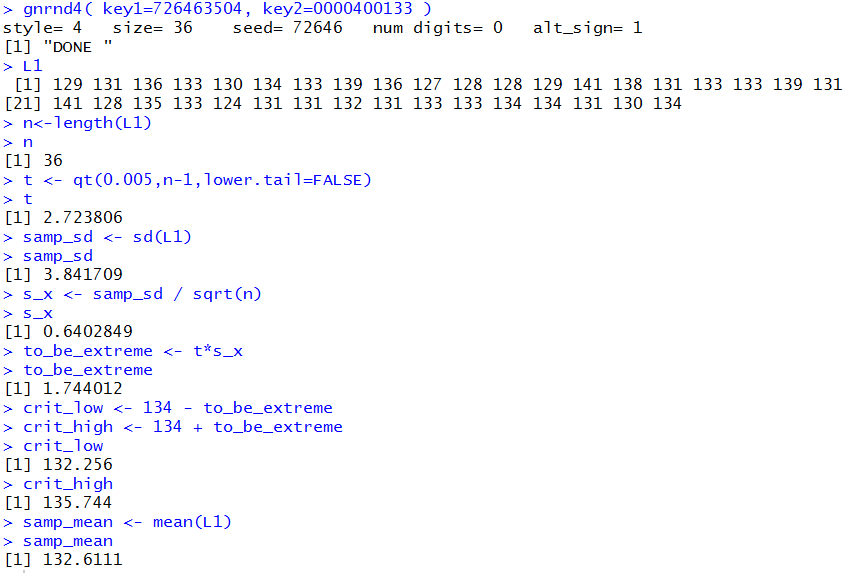
You should be able to reproduce these values in your R session. The result in this case is that the sample mean is not extreme enough to reject H₀.

The second static example is shown in Table 1b.
Figure 1b shows generating the table and making those computations in R.

Figure 1b

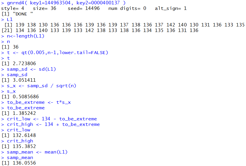
In this second static example the sample mean is greater than the upper critical value. Therefore, in this case we would reject H₀.

The presentation above walked us through the critical value approach for one dynamic and two static examples. Alternatively, you could use the attained significance approach. To do that, after determining that you are willing to make a Type I error 1% of the time, you take your 36-item sample. Starting with the dynamic example above, we already have that sample back in Table 1. You compute both the sample mean and the sample standard deviation for that data. We have that above, namely, , respecively. Following that you look to see just how likely it is to get a sample mean that extreme or more extreme from the 134 value assuming that H₀ is true, i.e., that the true population mean is 134.

You know that the distribution of 36-item sample means will be a Student's t with 35 degrees of freedom and will have a mean of 134 and a standard deviation of

The computations that we did above are pretty straight forward. We could do them based on the values stored in L1, in R using:

n<-length(L1)
n
samp_sd <- sd(L1)
samp_sd
s_x <- samp_sd / sqrt(n)
s_x
samp_mean <- mean(L1)
samp_mean
diff <- samp_mean - 134
diff
t<-diff/s_x
t
if( samp_mean < 134 ){
    p <- pt(t,35)
    pkind <- "lower"} else 
 {  p<-pt(t,35,lower.tail=FALSE)
    pkind <- "upper"}
pkind
p
p*2

You should note that the script included some "logic" to determine which of the two tails we should be using. The logic shown, the "if" construction, is sufficient in the case where we are using a "two-tailed" test. It will require some refinement later. Also, note that the script gives both a value for p and p*2. We still need to know which to use. In these "two-tailed" tests we will use the p*2 value.

After the dynamic example above, I included two static examples so that you could see the critical value script in action. We return to those same static examples to see the attained significance script in action.

The first static example was in Table 1a.
Figure 1a-attained shows generating that data and then making the R computations to use the attained significance approach.

Figure 1a-attained

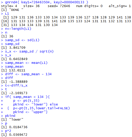
You should be able to reproduce these values in your R session. The result in this case is that the attained significance is not below the 0.01 level of the test so we cannot reject H₀.

The second static example is repeated in Table 1b.
Figure 1b-attained shows generating that data and then making the R computations to use the attained significance approach.

Figure 1b-attained

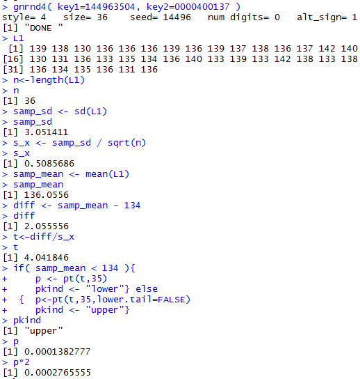
You should be able to reproduce these values in your R session. The result in this case is that the attained significance is below the 0.01 level of the test so we reject H₀.

Another dynamic example follows, this time with a bit less dialogue. We have a population which we know to be approximately normal. We do not know that the population standard deviation. There is a claim, a hypothesis, that the population mean is μ = 14.2, but we believe, for whatever reason, that the true population mean is higher than that. We want to test H₀: μ = 14.2 against the alternative H₁: μ > 14.2 at the 0.05 level of significance, meaning we are willing to make a Type I error one out of twenty times.

This is a "one-sided test" because the only time we will reject H₀ is if we get a sample mean significantly greater than the H₀ value of 14.2.

Because the population is normal we can get away with a smaller sample size. In fact, we decide to use a sample of size n=17. The distribution of 17-item sample means will be approximately Student's t with with 16 degrees of freedom and with standard deviation equal to approximately s/sqrt(17), where s is the sample standard deviation.

First we will do this with the critical value approach. The critical value we want needs to 5% of the area under the curve for the Student's t above it. On a standard student's t with 16 degrees of freedom, the t-value=1.746 has about 5% of the area above it. Our critical value will be 1.746*s above the null hypothesis mean of 14.2, but we cannot find our critical values until we know the value of s.

We take a sample, the values of which are shown in Table 2.

The computations that we did above are pretty straight forward. We could do them, excluding finding the sample mean, with a bit more accuracy, in R using:

n<-length(L1)
n
t <- qt(0.05,n-1,lower.tail=FALSE)
t
samp_sd <- sd(L1)
samp_sd
s_x <- samp_sd / sqrt(n)
s_x
to_be_extreme <- t*s_x
to_be_extreme
crit_high <- 14.2 + to_be_extreme
crit_high
samp_mean <- mean(L1)
samp_mean

We cannot demo those commands for the values in Table 2 because those values are dynamic, changing with each reload of the page. However, you should be able to use the gnrnd4() command above to create the same table and then run those commands to produce the same results that you see here.

To do this same problem using the attained significance approach we would ask "What is the probability that if H₀ is true we would find a random sample of 17 items with a sample mean that is

Here is a third example, one given with even less discussion.

We have a population and a null hypothesis H₀: μ = 239.7 with the alternative hypothesis H₁: μ < 239.7. We want to test H₀ at the 0.035 level of significance. We do not know the population standard deviation. There is a real concern that the population is not normally distributed. To address that concern we choose a sample size greater than 30. Our sample size will be n=68.

For the critical value approach, we note that the t-score for 67 degrees of freedom with the area 0.035 to its left is about -1.841. We take a random sample of 68 items. The values are reported in Table 3.

The computations that we did above are pretty straight forward. We could do them, excluding finding the sample mean, with a bit more accuracy, in R using:

n<-length(L1)
n
t <- qt(0.035,n-1)
t
samp_sd <- sd(L1)
samp_sd
s_x <- samp_sd / sqrt(n)
s_x
to_be_extreme <- t*s_x
to_be_extreme
crit_low <- 239.7 + to_be_extreme
crit_low
samp_mean <- mean(L1)
samp_mean

We cannot demo those commands for the values in Table 3 because those values are dynamic, changing with each reload of the page. Howver, you should be able to use the gnrnd4() command above to create the same table and then run those commands to produce the same results that you see here.

To do this same problem using the attained significance approach we would ask "What is the probability that if H₀ is true we would find a random sample of 68 items with a sample mean that is

The three dynamic (the samples change each time the page is reloaded or refreshed) examples above walk through problems of testing the null hypothesis for the population, where we do not know the population standard deviation, by drawing a sample and using either the critical value or the attained significance approach. In that "walking through" the problems we begin to recognize that the steps we will take are almost identical for each problem. We should be able to capture those steps in some R function. Consider the following function:

hypoth_test_unknown <- function(
  H0_mu,  H1_type=0, sig_level=0.05,
  samp_size, samp_mean, samp_sd)
{ # perform a hypothesis test for the mean=H0_mu
  # when we do not know sigma and the alternative hypothesis is
  #      !=  if H1_type==0
  #      <   if H1_type < 0
  #      >   if H1_type > 0
  # Do the test at sig_level significance, for a 
  # sample of size samp_size that yields a sample
  # mean = samp_mean and a sample standard deviation = samp_sd
  s_x <- samp_sd/sqrt(samp_size)
  if( H1_type == 0)
  { t <- abs( qt(sig_level/2,samp_size-1))}
  else
  { t <- abs( qt(sig_level,samp_size-1))}
  to_be_extreme <- t*s_x
  decision <- "Reject"
  if( H1_type < 0 )
    { crit_low <- H0_mu - to_be_extreme
      crit_high = "n.a."
      if( samp_mean > crit_low)
        { decision <- "do not reject"}
      attained <- pt( (samp_mean-H0_mu)/s_x, samp_size-1)
      alt <- paste("mu < ", H0_mu)
    }
  else if ( H1_type == 0)
  { crit_low <- H0_mu - to_be_extreme 
    crit_high <- H0_mu + to_be_extreme
    if( (crit_low < samp_mean) & (samp_mean < crit_high) )
        { decision <- "do not reject"}

    if( samp_mean < H0_mu )
      { attained <- 2*pt((samp_mean-H0_mu)/s_x,samp_size-1)}
    else
      { attained <- 2*pt((samp_mean-H0_mu)/s_x, samp_size-1,
                     lower.tail=FALSE)
      }
    alt <- paste( "mu != ", H0_mu)
  }
  else
    { crit_low <- "n.a."
      crit_high <- H0_mu + to_be_extreme
      if( samp_mean < crit_high)
        { decision <- "do not reject"}
      attained <- pt((samp_mean-H0_mu)/s_x, samp_size-1,
                 lower.tail=FALSE)
      alt <- paste("mu > ",H0_mu)
    }
  ts <- (samp_mean - H0_mu)/(samp_sd/sqrt(samp_size))
  result <- c(H0_mu, alt, s_x, samp_size, sig_level, t,
              samp_mean, samp_sd, ts, to_be_extreme,
              crit_low, crit_high, attained, decision)
  names(result) <- c("H0_mu", "H1:", "std. error", "n",
                     "sig level", "t"  ,"samp mean",  
                     "samp stdev", "test stat", "how far",
                     "critical low", "critical high",
                     "attained", "decision")
  return( result)
}

This is a long function, but it is really just the steps that we have taken in the previous examples. One of the things that make the function so long is that we have to build into it all of the "logic" that we apply to the problems as we do them. Thus, we had to build in the idea of splitting the significance level between both high and low values for the alternative hypothesis of being "not equal to". We also wanted to build in the process of deciding if we want to reject or not reject the null hypothesis.

As much as I would like to demonstrate how this function works for the dynamic examples above, I cannot do that here since those examples each contained random samples that change every time you load the page. However, I can repeat each of the static cases given above for the first dynamic situation, and follow that with two more static examples, one for each of the final two dynamic situations given above.

Revisit Example 1a:

We decided to take a 36-item sample. Then we found that the two critical values were 127.55 and 140.45. Then we took a sample shown in Table 1a above. From that sample we determined, in Figure 1a, that the sample mean is 132.6111 and the sample standard deviation is 3.841709. Recall that H₀ had μ=134, that this is a two-sided test, that the level of significance of the test is 1%, and that the sample size is 36. With all of that we can use our function via the command hypoth_test_unknown(134,0,0.01,36, 132.6111, 3.841709) as shown in Figure 2. Figure 2

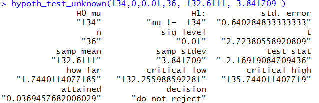
Figure 2 contains all of the results that we generated above for example 1a. It just does that as the result of one command. You might note that in order to construt that command we did need to knwo the sample size, the sample mean, and the sample standard deviation.

Revisit Example 1b:

We can do the same thing for example 1b. Here the command is just hypoth_test_unknown(134, 0, 0.01, 36, 136.0556, 3.051411 ) and the resulting output is shown in Figure 3.
Figure 3

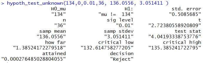
Again, the output includes all the values we had to construct above for example 1b.

A static example along the lines of example 2:

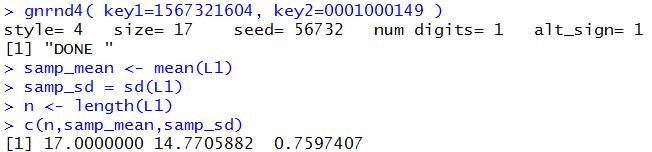
We have that same population, known to be normal, and we want to test H₀: μ = 14.2 against the alternative H₁: μ > 14.2 at the 0.05 level of significance. We take a sample of size 17 and get the values shown in Table 4. In order to perform our test in R we need to generate the sample there, find the sample sizze, mean , and standard deviation, and then formulate the command to run the hypoth_test_inknown() finction. The first part of that task can be done via

gnrnd4( key1=1567321604, key2=0001000149 )
samp_mean <- mean(L1)
samp_sd = sd(L1)
n <- length(L1)
c(n,samp_mean,samp_sd)

The results of that are shown in Figure 4.
Figure 4

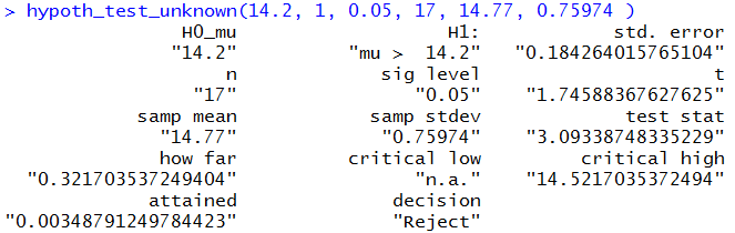
Once we know the values we can formulate the commad

hypoth_test_unknown(14.2, 1, 0.05, 17, 14.77, 0.75974 )

to produce the results shown in Figure 5.
Figure 5

The nice part of using the above approach is tht we get to see what is happening. However, because hypoth_test_unknown() gives us so much information, we could actually get this down to a more concise pair of statements, anmely,

gnrnd4( key1=1567321604, key2=0001000149 )
hypoth_test_unknown(14.2, 1, 0.05, 
                    length(L1), mean(L1), sd(L1) )

Which, together, produce the result shown in Figure 6.
Figure 6

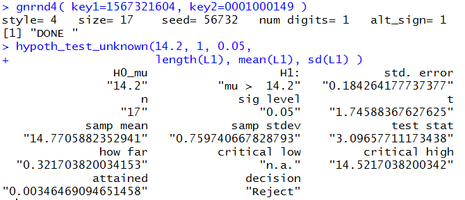
The result is the same, but the big advantage is that we did not have to type in the intermediate values. Furthermore, the statement of the function can be used again with a new problem where we need only change at most the first three parameters. For example, Table 5 holds a new sample for example 2.
We can perform the test on this sample via the commands

gnrnd4( key1=1321651604, key2=0001000145 )
hypoth_test_unknown(14.2, 1, 0.05,
                    length(L1), mean(L1), sd(L1) )

which produce the result shown in Figure 7.
Figure 7

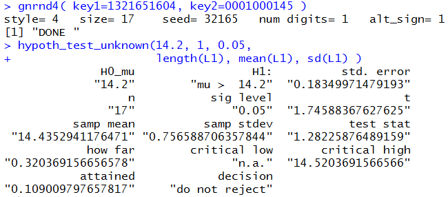
A different result, but there was very little change in the commands we used.

A static example along the lines of example 3:

We have that same population and we want to test H₀: μ = 239.7 against the alternative H₁: μ < 239.7 at the 0.035 level of significance. We take a sample of size 68 and get the values shown in Table 6.

Using the strategy that we just developed, we can generate the data and run the test via

gnrnd4( key1=1750376704, key2=0008302375 )
hypoth_test_unknown(239.7, -1, 0.035, 
                    length(L1), mean(L1), sd(L1) )

To generate the result shown in Figure 8.
Figure 8

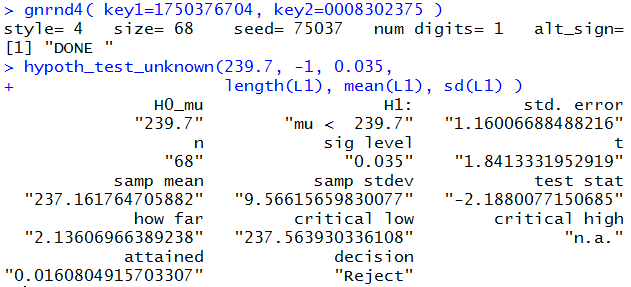
This seems to be a much more efficient solution to the problem than going through it as we did above for the dynamic version of the test.

Below is a listing of the R commands used in generating this page.

#critical value approach

gnrnd4( key1=726463504, key2=0000400133 )
L1
n<-length(L1)
n
t <- qt(0.005,n-1,lower.tail=FALSE)
t
samp_sd <- sd(L1)
samp_sd
s_x <- samp_sd / sqrt(n)
s_x
to_be_extreme <- t*s_x
to_be_extreme
crit_low <- 134 - to_be_extreme
crit_high <- 134 + to_be_extreme
crit_low
crit_high
samp_mean <- mean(L1)
samp_mean

gnrnd4( key1=144963504, key2=0000400137 )
L1
n<-length(L1)
n
t <- qt(0.005,n-1,lower.tail=FALSE)
t
samp_sd <- sd(L1)
samp_sd
s_x <- samp_sd / sqrt(n)
s_x
to_be_extreme <- t*s_x
to_be_extreme
crit_low <- 134 - to_be_extreme
crit_high <- 134 + to_be_extreme
crit_low
crit_high
samp_mean <- mean(L1)
samp_mean

gnrnd4( key1=302583504, key2=0000400135 )
L1
n<-length(L1)
n
t <- qt(0.005,n-1,lower.tail=FALSE)
t
samp_sd <- sd(L1)
samp_sd
s_x <- samp_sd / sqrt(n)
s_x
to_be_extreme <- t*s_x
to_be_extreme
crit_low <- 134 - to_be_extreme
crit_high <- 134 + to_be_extreme
crit_low
crit_high
samp_mean <- mean(L1)
samp_mean

# attained approach 

gnrnd4( key1=726463504, key2=0000400133 )
L1
n<-length(L1)
n
samp_sd <- sd(L1)
samp_sd
s_x <- samp_sd / sqrt(n)
s_x
samp_mean <- mean(L1)
samp_mean
diff <- samp_mean - 134
diff
t<-diff/s_x
t
if( samp_mean < 134 ){
  p <- pt(t,35)
  pkind <- "lower"} else 
  {  p<-pt(t,35,lower.tail=FALSE)
  pkind <- "upper"}
pkind
p
p*2



gnrnd4( key1=1833071604, key2=0001000150 )
L1
n<-length(L1)
n
samp_sd <- sd(L1)
samp_sd
s_x <- samp_sd / sqrt(n)
s_x
samp_mean <- mean(L1)
samp_mean
diff <- samp_mean - 134
diff
t<-diff/s_x
t
if( samp_mean < 134 ){
    p <- pt(t,35)
    pkind <- "lower"} else 
 {  p<-pt(t,35,lower.tail=FALSE)
    pkind <- "upper"}
pkind
p
p*2

# second dynamic example

gnrnd4( key1=1833071604, key2=0001000150 )
L1
n<-length(L1)
n
t <- qt(0.05,n-1,lower.tail=FALSE)
t
samp_sd <- sd(L1)
samp_sd
s_x <- samp_sd / sqrt(n)
s_x
to_be_extreme <- t*s_x
to_be_extreme
crit_high <- 14.2 + to_be_extreme
crit_high
samp_mean <- mean(L1)
samp_mean
diff <- samp_mean - 14.2
diff
t<-diff/s_x
t
if( samp_mean < 14.2 ){
  p <- pt(t,16)
  pkind <- "lower"} else 
  {  p<-pt(t,16,lower.tail=FALSE)
  pkind <- "upper"}
pkind
p
p*2


gnrnd4( key1=1277746704, key2=0005002380 )
n<-length(L1)
n
t <- qt(0.035,n-1)
t
samp_sd <- sd(L1)
samp_sd
s_x <- samp_sd / sqrt(n)
s_x
to_be_extreme <- t*s_x
to_be_extreme
crit_low <- 239.7 + to_be_extreme
crit_low
samp_mean <- mean(L1)
samp_mean
diff <- samp_mean - 239.7
diff
t<-diff/s_x
t
if( samp_mean < 239.7 ){
  p <- pt(t,67)
  pkind <- "lower"} else 
  {  p<-pt(t,67,lower.tail=FALSE)
  pkind <- "upper"}
pkind
p
p*2

source("../hypo_unknown.R")

# revisit 1a
hypoth_test_unknown(134,0,0.01,36, 132.6111, 3.841709 )
# revisit 1b
hypoth_test_unknown(134, 0, 0.01, 36, 136.0556, 3.051411 )
#static sample for example 2
gnrnd4( key1=1567321604, key2=0001000149 )
samp_mean <- mean(L1)
samp_sd = sd(L1)
n <- length(L1)
c(n,samp_mean,samp_sd)
hypoth_test_unknown(14.2, 1, 0.05, 17, 14.77, 0.75974 )
# or done in just two statements
gnrnd4( key1=1567321604, key2=0001000149 )
hypoth_test_unknown(14.2, 1, 0.05, 
                    length(L1), mean(L1), sd(L1) )


gnrnd4( key1=1321651604, key2=0001000145 )
hypoth_test_unknown(14.2, 1, 0.05, 
                    length(L1), mean(L1), sd(L1) )

gnrnd4( key1=1750376704, key2=0008302375 )
hypoth_test_unknown(239.7, -1, 0.035, 
                    length(L1), mean(L1), sd(L1) )

hypoth_test_known(239.7, 43.6, -1, 0.035, 68, 230.028 )