Hypothesis Test for Population Standard Deviation for normal population

Return to Topics page
The situation is:

We have a population that is normally distributed. For this situation it is important that the population has a normal distribution but we do not need to know, ahead of time, the mean or standard deviation of that distribution.
We are interested in the standard deviation, σ, of the population.
We have a hypothesis about the "true" value of the population standard deviation. That is, someone (perhaps us) claims that H₀: σ = a, for some value a.
We will consider an alternative hypothesis which is one of the following
- H₁: σ > a,
- H₁: σ < a, or
- H₁: σ ≠ a.
We want to test H₀ against H₁.
We have already determined the level of significance that we will use for this test. The level of significance, α, is the chance that we are willing to take that we will make a Type I error, that is, that we will reject H₀ when, in fact, it is true.

Immediately, we recognize that samples of size n drawn from this population will have a distribution of the ratio of n-1 times the sample variance to the population variance that is a χ² with n-1 degrees of freedom. Thus, if H₀ is true and the population standard deviation is a, then for samples of size n the statistic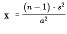

will have a χ² distribution with n-1 degrees of freedom.

At this point we proceed via the critical value approach or by the attained significance approach. These are just different ways to create a situation where we can finally make a decision. The critical value approach tended to be used more often when everyone needed to use the tables. The attained significance approach is more commonly used now that we have calculators and computers to do the computations. Of course either approach can be done with tables, calculators, or computers. Either approach gives the same final result.

We determine a sample size n. This will set the number of degrees of freedom as we use the χ² distribution.

Critical Value Approach

Find the value or values (depending upon if we are looking at a one-tailed or a two-tailed test) of χ² that have the level of significance area outside of the value or values. For a two-tailed test (H₁: σ ≠ a) we need to split the level of significance so that half is at the low end and half is at the right end. [This is made somewhat more complex if you are using a table since most tables only give the upper tail value and because χ² is not a symmetric distribution.] Use that value or those values as the critical values.
Take the random sample of size n and compute the sample standard deviation, s, from that sample.
Compute the value .
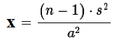If that value is beyond the critical value(s) then we say that "we reject H₀ in favor of the alternate H₁". If that value is not more extreme than the critical value(s) then we say "we have insufficient evidence to reject H₀".

Attained significance Approach

We compute the sample standard deviation, s.
Compute .
Using the χ² distribution, and taking into account the alternative hypothesis, H₁, so that we know if we are doing a one-tail or two-tail test, we compute the probability of getting the value χ2 or a value more extreme than that.
If the resulting probability is smaller than or equal to the predetermined level of significance then we say that "we reject H₀ in favor of the alternate H₁". If the resulting probability is not less than the predetermined level of significance then we say "we have insufficient evidence to reject H₀".

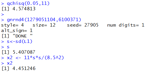
We will work our way through an example to see this. Assume that we have a normal population of values. I claim that the true standard deviation, σ of those values is 8.5. You suspect that the true standard deviation is not 8.5 but rather some value less than that. We agree to test the null hypothesis H₀: σ = 8.5 against the alternative hypothesis H₁: σ < 8.5 at the 0.05 level of significance. To do this we agree to take a random sample of size 12 from the population and then compute the sample standard deviation, s. If s is far enough below 8.5 we will reject H₀ in favor of H₁. The question is, how far below 8.5 is far enough so that if the null hypothesis is true then we will reject it no more than 5% of the time based upon a sample of size 12?

The critical value approach has us look to the χ² distribution for n-1, that is 11 degrees of freedom and to find the χ² value that has 5% of the area under the curve to the left of that value. We could use a table, a calculator, or the computer to get this. The result is the value 4.575, rounded to 3 decimal places.

Remember, 4.575 is the χ² value. We need to compute the test statistic from

and compare that value against 4.575.

We take a sample, shown in Table 1. If we assign that value to s then we can compute our test statistic as 11*s*s/(8.5^2), which turns out to be about 4.451, a value that is less than our critical value of 4.575. Therefore, based on that sample, we reject H₀ in favor of H₁ at the 0.05 level of significance.

The computations that we did above are shown in Figure 1.

Figure 1

To do the same problem using the attained significance approach, we take our sample of size 12 shown in Table 1, we find the sample standard deviation which we found to be s=5.407087, we compute our test statistic, x2=4.451246 and then we find the area under the curve to the left of that value for 11 degrees of freedom. The R command to do this is pchisq(x2,11). If that value is less than our predetermined level of significance, in this case 5%, then we reject H₀. The console view of the command is shown in Figure 2.

Figure 2

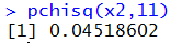
Indeed, the result is 0.045 which is less than the 5% significance level for the problems. Therefore, we reject H₀ just as we did using the critical value approach.

In all fairness, I wanted to demonstrate such a rejection. As such, I created a call to gnrnd4() that I knew woud produce the result that I wanted to use as an example. Table 2 gives more a more fair sample. It really is drawn from a population that has a standard deviation of 8.5. Of course, each time this page is reloaded we get a new sample in Table 2. Therefore, you could repeatedly refresh this page and see how the values of the sample standard deviation, s, and the test statistic, x2, change with each new sample. Furthermore, using the critical value approach, we know that we will reject H₀ about 5% of the time.

A second example:

We assume that we have a normal population of values and that the null hypothesis is that the standard deviation of the population is 24.38. The alternative hypothesis is that the true population standard deviation is greater than 24.38. We want to test the null hypothesis, H₀: σ = 24.38, against the alternative hypothesis, H₁: σ > 24.38, at the 0.025 level of significance. We decide to take samples of size 22.

For the critical value approach we use the fact that if we take samples of size 22, compute the sample standard deviation, s, for each sample, then compute

for each such sample, the value x will have a χ² distribution with 21 degrees of freedom. From the χ² tables or from a calculator or from the computer we determine that at 21 degrees of freedom the χ² value 35.479 has 2.5% of the area under the curve to its right. Therefore, we set our critical value at 35.479.

Next we take a random sample. Our sample is shown in Table 3.

A third example:

We assume that we have a normal population of values and that the null hypothesis is that the standard deviation of the population is 3.25. The alternative hypothesis is that the true population standard deviation is not equal to 3.25 . We want to test the null hypothesis, H₀: σ = 3.25, against the alternative hypothesis, H₁: σ ≠ 3.25, at the 0.0333 level of significance. Note that this is a two-tailed test. We will reject H₀ if our sample standard deviation is either too high or too low. We will need χ² values that give us 1.6666% of the area below the low value and 1.6666% of the area above to high value. We decide to take samples of size 15.

For the critical value approach we use the fact that if we take samples of size 15, compute the sample standard deviation, s, for each sample, then compute

for each such sample, the value x will have a χ² distribution with 14 degrees of freedom. From the χ² tables or from a calculator or from the computer we determine that at 14 degrees of freedom the χ² value 5.1676 has 1.6666% of the area under the curve to its left, while the χ² value 27.4809 has 1.6666% of the area under the curve to its right, Therefore, we set our critical values at 5.1676 and 27.4809.

Next we take a random sample. Our sample is shown in Table 4.

Using the attained significance approach in this last example was a bit more tricky. If you reload this page a number of times you will see that the R command that we used changed, as needed, between pchisq(x2,14) and pchisq(x2,14,lower.tail=FALSE). Our sample gives a sample standard deviation that is either lower than or higher than the H₀ value, 3.25. If it is lower then we need to ask is it low enough to reject H₀. If it is higher then we need to ask is it high enough to reject H₀. Thus, depending on the sample standard deviation we need to choose which tail we want to use, and that determines the form of the pchisq() command to use. We will take that into account below when we formulate a function to do all of this in one step.

The following function definition for hypoth_test-sigma() incorporates all of the steps for the various cases that we have seen above. The file that holds this function is available for download at hypo_sigma.R.

# Roger Palay copyright 2016-02-08
# Saline, MI 48176
#
hypoth_test_sigma <- function(
       H0_sigma,  n, samp_sigma, H1_type, sig_level=0.05)
{ # perform a hypothsis test for the population
  # standard deviation=H0_sigma
  # based on a sample of n items yielding a
  # sample standard deviation, samp_sigma,
  #  where the alternative hypothesis  is
  #      !=  if H1_type==0
  #      <   if H1_type < 0
  #      >   if H1_type > 0
  # Do the test at sig_level significance,
  #
  # It is important that the population is a normal
  # distribution.

  decision <- "Reject"
  x2 <- (n-1)*(samp_sigma^2)/(H0_sigma^2)
  if( H1_type < 0 )
    { crit_low <- qchisq( sig_level, n-1 )
      crit_high <- "n.a."
      if( x2 > crit_low )
         { decision <- "Do Not Reject" }
      attained <- pchisq( x2, n-1 )
      alt <- paste("sigma < ", H0_sigma)
    }
  else if( H1_type > 0 )
    { crit_high <- qchisq( sig_level, n-1, lower.tail=FALSE )
      crit_low <- "n.a."
      if( x2 < crit_high )
         { decision <- "Do Not Reject" }
      attained <- pchisq( x2, n-1, lower.tail=FALSE )
      alt <- paste("sigma > ", H0_sigma)
    }
  else
    { crit_low <- qchisq( sig_level/2, n-1 )
      crit_high <- qchisq( sig_level/2, n-1, lower.tail=FALSE )
      if (x2 >crit_low & x2 < crit_high )
         { decision <- "Do Not Reject" }
      if( samp_sigma < H0_sigma )
        { attained =2*pchisq( x2, n-1 ) }
      else
        { attained =2*pchisq( x2, n-1, lower.tail=FALSE ) }
      alt <- paste("sigma != ", H0_sigma)
    }
  result <- c(H0_sigma,  n, samp_sigma, alt, sig_level,
              crit_low, crit_high, x2, attained,
              decision)
  names(result) <- c("H0_sigma","Sample Size", 
              "Samp Sigma", "H1", "sig level",
              "crit low","crit high","chi2 val",
              "attained","Decision")
  return( result )
}

Table 5 gives six illustrations of problems involving hypothesis testing for the popultion standard deviation.

Table 5: Case studies
Case	H₀	Sample Size	Sample Standard Deviation	H₁	Level of Significance
I	H₀: σ = 4.63	16	3.24	H₁: σ < 4.63	0.075
II	H₀: σ = 4.63	16	3.57	H₁: σ < 4.63	0.075
III	H₀: σ = 18.43	32	22.52	H₁: σ > 18.43	0.02
IV	H₀: σ = 18.43	32	23.45	H₁: σ > 18.43	0.02
V	H₀: σ = 7.35	28	5.78	H₁: σ ≠ 7.35	0.08
VI	H₀: σ = 7.35	41	5.78	H₁: σ ≠ 7.35	0.08

To perform the hypothesis test for Case I we use the command

hypoth_test_sigma( 4.63, 16, 3.24, -1, 0.075)

Figure 3 holds the console image of this command.

Figure 3

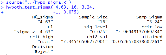
This is a one tail test using the lower tail. Using the critical value approach we find that the critical value is 7.9695. The computed statistic is 7.345, which is even lower than the critical value. Therefore we reject H₀.

Using the attained significance approach, we find the attained significance is 0.0526 which is less than the given significance level of 0.075. Therefore we reject H₀.

To perform the hypothesis test for Case II we use the command

hypoth_test_sigma( 4.63, 16, 3.57, -1, 0.075)

Figure 4 holds the console image of this command.

Figure 4

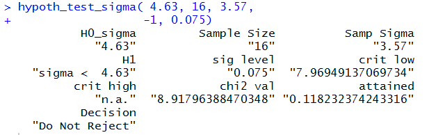
This is a one tail test using the lower tail. Using the critical value approach we find that the critical value is 7.9695. The computed statistic is 8.918, which is higher than the critical value. Therefore we do not reject H₀.

Using the attained significance approach, we find the attained significance is 0.1182 which is greater than the given significance level of 0.075. Therefore we do not reject H₀.

To perform the hypothesis test for Case III we use the command

hypoth_test_sigma( 18.43, 32, 22.52, 1, 0.02)

Figure 5 holds the console image of this command.

Figure 5

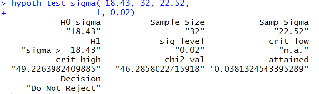
This is a one tail test using the upper tail. Using the critical value approach we find that the critical value is 49.226. The computed statistic is 46.258, which is lower than the critical value. Therefore we do not reject H₀.

Using the attained significance approach, we find the attained significance is 0.03813 which is greater than the given significance level of 0.02. Therefore we do not reject H₀.

To perform the hypothesis test for Case IV we use the command

hypoth_test_sigma( 18.43, 32, 23.45, 1, 0.02)

Figure 6 holds the console image of this command.

Figure 6

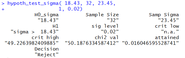
This is a one tail test using the upper tail. Using the critical value approach we find that the critical value is 49.226. The computed statistic is 50.1876, which is higher than the critical value. Therefore we reject H₀.

Using the attained significance approach, we find the attained significance is 0.016 which is less than the given significance level of 0.02. Therefore we reject H₀.

To perform the hypothesis test for Case V we use the command hypoth_test_sigma( 7.35, 28, 5.78, 0, 0.06) Figure 7 holds the console image of this command.

Figure 7

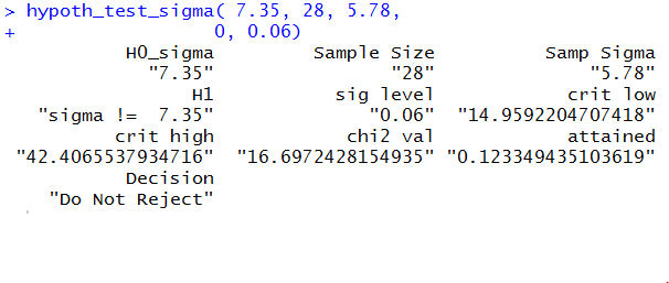
This is a two tail test using both a lower and upper tail, each having half of the area specified by the level of significance. Using the critical value approach we find that the critical values are 14.959 and 42.4066. The computed statistic is 16.697, which is between the critical values. Therefore we do not reject H₀.

Using the attained significance approach, we find the attained significance is 0.123 which is greater than the given significance level of 0.06. Therefore we do not reject H₀.

To perform the hypothesis test for Case VI we use the command

hypoth_test_sigma( 7.35, 41, 5.78, 0, 0.06)

Figure 8 holds the console image of this command.

Figure 8

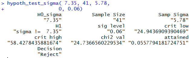
This is a two tail test using both a lower and upper tail, each having half of the area specified by the level of significance. Using the critical value approach we find that the critical values are 24.94379 and 58.4278. The computed statistic is 24.7367, which is not between the critical values. Therefore we reject H₀.

Using the attained significance approach, we find the attained significance is 0.0558 which is less than the given significance level of 0.06. Therefore we reject H₀.

Below is a listing of the R commands used in generating this page.

source("../gnrnd4.R")

qchisq(0.05,11)

gnrnd4( key1=1279051104, key2=0006100371 )
gnrnd4( key1=1500541104, key2=0008500578 )
s<-sd(L1)
s
x2 <- 11*s*s/(8.5^2)
x2
pchisq(x2,11)

qchisq(0.025,21,lower.tail=FALSE)

# sample that rejects the null hypothesis
gnrnd4( key1=2787062104, key2=0243819982 )
L1
s<-sd(L1)
s
x2 <- 21*s*s/(24.38^2)
x2
pchisq(x2,21,lower.tail=FALSE)

#  another sample that rejects the null hypothesis
gnrnd4( key1=2332182104, key2=0243840658 )
L1
s<-sd(L1)
s
x2 <- 21*s*s/(24.38^2)
x2
pchisq(x2,21,lower.tail=FALSE)

#   sample that does not reject the null hypothesis
gnrnd4( key1=2864272104, key2=0243844528 )
L1
s<-sd(L1)
s
x2 <- 21*s*s/(24.38^2)
x2
pchisq(x2,21,lower.tail=FALSE)

qchisq(0.01666, 14)
qchisq(0.01666, 14, lower.tail=FALSE)


# sample that rejects the null hypothesis
# for two-tailed test at 0.03333 level
gnrnd4( key1=2791411404, key2=0032524217 )
L1
s<-sd(L1)
s
x2 <- 14*s*s/(3.25^2)
x2
pchisq(x2,14)
pchisq(x2,14,lower.tail=FALSE)


# sample that does not reject the null hypothesis
# for two-tailed test at 0.03333 level
gnrnd4( key1=2364551404, key2=0032515898 )
L1
s<-sd(L1)
s
x2 <- 14*s*s/(3.25^2)
x2
pchisq(x2,14)
pchisq(x2,14,lower.tail=FALSE)

source("../hypo_sigma.R")
hypoth_test_sigma( 4.63, 16, 3.24, 
                  -1, 0.075)

hypoth_test_sigma( 4.63, 16, 3.57, 
                  -1, 0.075)

hypoth_test_sigma( 18.43, 32, 22.52, 
                 1, 0.02)

hypoth_test_sigma( 18.43, 32, 23.45, 
                 1, 0.02)

hypoth_test_sigma( 7.35, 28, 5.78, 
                 0, 0.06)


hypoth_test_sigma( 7.35, 41, 5.78, 
                 0, 0.06)