Hypothesis Test for Population Proportion
Return to Topics page
The situation is:
- We have a population the members of which fall into two groups,
those with a particular characteristic and those without that
characteristic. (As a small aside, the population may fall
into many groups but we focus on one characteristic and
lump the rest into a group of items not having that characteristic.)
- We are interested in the proportion, p, of the population
with the particular characteristic.
- We have a hypothesis about the "true" value of the population proportion.
That is, someone (perhaps us) claims that
H0: p = a,
for some value a.
- We will consider an alternative hypothesis which is one of the following
- H1: p > a,
- H1: p < a, or
- H1: p ≠ a.
- We want to test
H0 against H1.
- We have already determined
the level of significance that we will use for this test.
The level of significance, α,
is the chance that we are willing to take that
we will make a Type I error,
that is, that we will reject H0
when, in fact, it is true.
|
|
Immediately, we recognize that samples
of size n drawn from this population
with have a distribution of the
sample proportion that is a
normal with mean=p and
standard deviation=sqrt(p*(1-p)/n).
At this point we proceed via
the critical value approach
or by the attained significance approach.
These are just different ways to
create a situation where we can finally make a decision.
Of the two, the
attained significance approach is more commonly
used. Either approach gives the same final result.
|
|
Critical Value Approach
- Using the normal distribution we find the z-score that corresponds to
having the level of significance area more extreme than that z-score,
remembering that if we are looking at being either too low or too high
then we need half the area in both extremes.
- We determine a sample size n.
In doing this we need to be sure that both (n)(p)≥10 and
(n)(1-p)≥10.
- Also, we cannot sample more than 5% of the population.
That means that the size of the population must be more than 20 times n.
- Compute
 and use that value to
compute
and use that value to
compute  . .
- Set the critical value (or values in the case of a two-sided test)
such that it (they) mark the value(s) that is (are) that distance,
,
away from the proportion given
by H0: p = a.
- Then, we take a random sample of size n from the population.
- We compute the sample proportion,
 . .
- If that proportion
is more extreme than the critical value(s)
then we say that
"we reject H0 in favor of
the alternate H1". If the
sample proportion
is not more extreme than the critical value(s)
then we say "we have insufficient
evidence to reject H0".
| |
Attained significance Approach
- We determine a sample size n.
In doing this we need to be sure that both (n)(p)≥10 and
(n)(1-p)≥10.
- Also, we cannot sample more than 5% of the population.
That means that the size of the population must be more than 20 times n.
- Then, we take a random sample of size n from the population.
- We compute the sample proportion, .
- Compute
.
- Compute
 . .
- Using the standard normal distribution,
and taking into account the alternative hyposthesis,
H1, so that we know
if we are doing a one-tail or two-tail
test,
we compute the probability of getting the value
z or a value more extreme than that.
- If the resulting probability is smaller than or equal to the
predetermined level of significance then we say that
"we reject H0 in favor of
the alternate H1". If the
resulting
probability is not less than the predetermined level of significance
then we say "we have insufficient evidence to reject H0".
|
We will work our way through an example to see this.
Assume that we have a population of values
and that the members of that population fall into two groups, those
with a certain characteristic and those without that characterisitic.
In fact we will look at the population of M&M's in standard party packages
of the candy. We will look at the proportion
of the candies that are Green.
Although it is true that there are 5 other colors
of the candies (Red, Brown, Blue, Orange, and Yellow)
we lump all those togethere as non-Green.
Thus any particuar candy is either Green or non-Green.
I claim that the proportion of the population
that is Green is 21%.
That is, I claim that H0: p=0.21 is true.
You do not believe me.
You think the proportion of the population that is Green is
not equal to 21%.
That is, you believe that H1: p≠0.21 is true.
Notice that you are not saying what the true proportion is, just that
it is not 21%.
In order to test this difference of opinions, we
agree to take a sample of size 75 from a large bin of M&M's that
holds well over 4000 of the candies assembled from a random sample of party bags of
M&M's. The size of the sample is important.
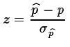
We note that 75*0.21 = 15.75 ≥ 10
and 75*(1-0.21) = 59.25 ≥ 10.
Furthermore, 75/4000 = 0.01875 so we
are clearly sampling less than 5% of the population.
If the null hypothesis is true, p = 0.21, we know that the
distribution of sample proportions from samples of size 75 will be
sqrt(p*(1-p)/n) = sqrt(0.21*(1-0.21)/75) ≈0.0470319.
Critical value approach:
Our level of significance is 0.05.
However, this is a two-tailed test
(an extreme value either higher or lower than 0.21 would
indicate that the null hypothesis is false).
Therefore, we want to find, in the standard normal distribution,
values for z that have 0.025 square units to the left of one value and 0.025
square units to the right of the other value.
We could use the table, a calculator, or the computer to find those values.
They turn out to be about -1.96 and 1.96, respectively.
Figure 1 shows all the calculatorions that we have done so far.
Figure 1
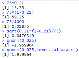
Then we can find the
critical values by finding the proportions that are
z*σ away from the null hypothesis value, p.
The calculations to do this are
sigma <- sqrt(0.21*(1-0.21)/75)
z_left <- qnorm(0.025)
z_right <- qnorm(0.025,lower.tail=FALSE)
crit_low <-0.21 + z_left*sigma
crit_high <- 0.21 + z_right * sigma
crit_low
crit_high
The console view of those commands shown in Figure 2.
Figure 2
The result is that our critical values are
0.1178 and 0.3022.
Now we take our actual sample, shown in Table 1
where the candy colors, Red, Green, Brown, Blue, orange, and Yellow,
are represented by the values 1, 2, 3, 4, 5, and 6, respectively.
Now we need to find the proportion of the
candies in the sample that are Green.
To do this we count the number of 2's in the table.
There are 10 such candies.
The commands to generate the data, verify the data,
and
get the desired count, first using the built-in
table() function and second using our
make_freq_table() function are:
gnrnd4(623127407,6997566)
L1
table(L1)
make_freq_table(L1)
The console view of those commands shown in Figure 3.
Figure 3
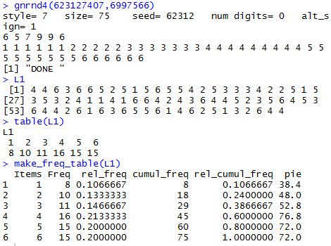
Knowing that there are 10 Green candies out of 75
candies in the sample means that the proportion of
Green candies is 10/75 or 0.1333,
a value we would compute as 10/75 using the table() output
or that we can read directly from the
make_freq_table() output.
Thus, =0.1333, a value that is neither below our
low
critical value, 0.1178 nor above our high
critical value, 0.3022.
Therefore we would conclude that we do not have sufficient
evidence to reject H0 at
the 0.05 level of significance.
Attained significance approach:
In this approach we still compute
σ=sqrt(p*(1-p)/n), and we still take
our sample, shown in Table 1, and
we still compute .
However, at that point we compute
.
Then using that value we find the area
that is further away from 0.21 than that value of z.
In this case, because this is a two-tail test,
we need to add the area that is on the right, further away from
0.21 than our value of z
was away on the left. But, we know that the distribution
is normal and a normal distribution is symmetric.
Therefore, the area on the right will be the same as
the area on the left.
To get the sum of the two areas
we just need to double the area we found on the left.
These computations are:
sigma <- sqrt(0.21*(1-0.21)/75)
z <- (10/75-0.21)/sigma
# since the proportion is lower than 0.21
# look at the left tail
prob <- pnorm(z)
prob
prob*2
The console view of those commands shown in Figure 4.
Figure 4
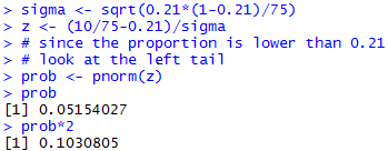
From Figure 4 we see that the
attained significance was 0.103,
a value not less than the level of significance, 0.05,
for the test.
Therefore, we say we do not have sufficient
evidence to reject the null hypothesis.
Changed problem:
Above we used a 5% level of significance. That meant that we were
willing to make a Type I error 5% of the time.
That is, even if H0: p = 0.21
is correct, if were repeat this process of taking samples of size 75
and base our decision to reject H0 or
to not reject it on the proportion of Green candies in the sample,
then we expect to incorrectly reject H0
about 5% of the time, that is, on average, 1 out of 20 times.
Now, look at the problem again, but this time we are willing
to make a Type I error 12.5% of the time,
on average, 1 out of 8 times.
Using the same sample, the data in Table 1 we would have
to redo some of the calculations
for the critical value approach. In particular, we would need
to do the calculations:
sigma <- sqrt(0.21*(1-0.21)/75)
z_left <- qnorm(0.0625)
z_right <- qnorm(0.0625,lower.tail=FALSE)
crit_low <-0.21 + z_left*sigma
crit_high <- 0.21 + z_right * sigma
crit_low
crit_high
The console view of these commands appears in Figure 5.
Figure 5
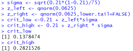
The computation of sigma in Figure 5 is
just a repeat of our earlier computation, first shown in Figure 2.
The other computations are modified to get the two-tail values
for the total of 0.125 square units outside the z-values,
and then the computation of the actual critical values.
In this changed problem, because our sample produced a proportion of
0.1333 which is less than the new lower critical value, 0.1378,
we would reject H0 at the 0.125 level
in favor of H1.
You might note that using the attained siginificance approach
we would still be using the information in Figure 4 and we would say that
the attained significance 0.1031 is less than the new level, 0.125
so we would reject H0 at the 0.125 level
in favor of H1.
A new problem:
We have a population of size 950 where some items in the population have
with a characteristic and the rest do not.
We have a null hypothesis that the proportion of the population that has that
characterisitic is 0.25, that is 1 out of 4.
We have an alternative hypothesis that the true proportion
is greater than 0.25.
We want to test H0: p = 0.25
against H1: p > 0.25 at the
0.0625 level of significance. This is a one-tail test.
When we get around to taking a sample, in order to justify rejecting
H0 in favor of H1
we will need to find the proportion of the sample with the characteristic
to be significantly higher than 0.25.
If we were to find the proportion in the sample to be 0.08
that might indicate that the 0.25 was wrong,
but it would not suggest that the true value is actually higher
than the 0.25 value.
We follow the same steps as we did above, except that this is a one-tail test.
We decide on a sample size, n. We know that we need 0.25*n≥10
and (1-0.25)*n≥10.
To meet that requirement, the smallest sample size that we can use is 40.
To meet the requirement that we not sample more than 5%
of the population we need to keep the sample size less than or equal to
0.05*950 = 47.5. We will settle on a sample size of
n=45 to meet both restrictions.
For the critical value approach we can start with the computations:
sigma <- sqrt(0.25*(1-0.25)/45)
sigma
z_right <- qnorm(0.0625,lower.tail=FALSE)
crit_high <- 0.25 + z_right * sigma
crit_high
The console view of these appears in
Figure 6.
Figure 6
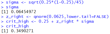
From Figure 6 we see that the critical value is 0.349.
Thus, when we take our sample of size 45 if the proportion of
items with the specified characteristic is 0.349 or higher then we will
reject the null hypothesis.
We take our random sample and find that it is the values given in
Table 2.
|
Just as a point of information, the specification of gnrnd4()
used to produce Table 2 asks that function to produce a sample
from a
population that has 25% of the values having the characteristic.
Now, gnrnd4() may not be perfect, but it does a reasonably good job
of fullfilling that task. Therefore, if you reload this page over and over you
should see that we do reject H0 about 6.25% of the time
when it is really true.
|
Because we have different values for
each time we load the page, I cannot show you the exact R
statements to compute the
attained significance in this dynamic example.
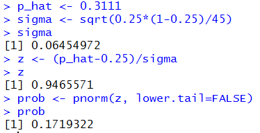
However, if the proportion was found to be 0.3111,
the result of finding 14 of the 45 items having the characteristic,
then we would use the
commands:
p_hat <- 0.3111
sigma <- sqrt(0.25*(1-0.25)/45)
sigma
z <- (p_hat-0.25)/sigma
z
prob <- pnorm(z, lower.tail=FALSE)
prob
which would produce the console output shown in Figure 7.
Figure 7
I can tell you that for the specific sample shown in Table 2
where the proportion is
Yet another new problem:
We have a population of size 7589 where some
items in the population have
with a characteristic and the rest do not.
We have a null hypothesis that the proportion of
the population that has that
characterisitic is 0.7, that is 7 out of 10.
We have an alternative hypothesis that the true proportion
is less than 0.7.
We want to test H0: p = 0.7
against H1: p < 0.7
at the
0.03 level of significance. This is a one-tail test.
When we get around to taking a sample, in order to justify rejecting
H0 in favor of
H1
we will need to find the proportion of the sample
with the characteristic
to be significantly lower than 0.7.
If we were to find the proportion in the sample to be 0.85
that might indicate that the 0.7 was wrong,
but it would not suggest that the true value is actually lower
than the 0.7 value.
We follow the same steps as we did above, except that this is a one-tail test.
We decide on a sample size, n. We know that we need 0.7*n≥10
and (1-0.7)*n≥10.
To meet that requirement, the smallest
sample size that we can use is 34.
To meet the requirement that we not sample more than 5%
of the population we need to keep the sample size less than or equal to
0.05*7589 = 379.45.
This should not be a problem.
We will settle on a sample size of
n=35, a value that meets both restrictions.
For the critical value approach we can start with the computations:
sigma <- sqrt(0.7*(1-0.7)/35)
sigma
z_left <- qnorm(0.03)
z_left
crit_low <- 0.7 + z_left * sigma
crit_low
The console view of some of our preliminary computations
along with these commands appears in
Figure 8.
Figure 8
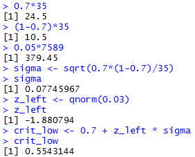
From Figure 8 we see that the critical value is 0.5543.
Thus, when we take our sample of size 35 if the proportion of
items with the specified characteristic is 0.5543 or lower then we will
reject the null hypothesis.
We take our random sample and find that it is the values given in
Table 3.
Because we have different values for
each time we load the page, I cannot show you the exact R
statements to compute the attained significance in this dynamic example.
However, if the proportion was found to be 0.6,
corresponding to having 21 of the items be a 2, then we would use the
commands:
p_hat <- 0.6
sigma <- sqrt(0.7*(1-0.7)/35)
sigma
z <- (p_hat-0.7)/sigma
z
prob <- pnorm(z)
prob
which would produce the console output shown in Figure 9.
Figure 9
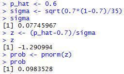
I can tell you that for the specific sample shown in Table 3
where the proportion is
We have seen that we can use either the critical value or the attained
significance approach to perform a test for the population proportion.
There are not that many steps to either approach, but as has been the case in
earlier hypothesis test pages, we might as well capture these steps in a
function that we define in R.
The quatities or directions tht we need to know to do the test are
- the proportion stated in H0
- the number of items in the sample that have the characteristic
- the number of items in the sample
- an indication of the statement of the alternative hypothesis,
i.e., is it stated as
≠, <, or >
- the specified level of significance.
If we have all of that then we can just go ahead and compute the result.
Consider the following function:
# Roger Palay copyright 2016-01-31
# Saline, MI 48176
#
hypoth_test_prop <- function(
       H0_p, x, n, H1_type, sig_level=0.05)
{ # perform a hypothsis test for the proportion=H0_p
  # based on finding x items out of the n items in
  # the sample, where the alternative hypothesis  is
  #      !=  if H1_type==0
  #      <   if H1_type < 0
  #      >   if H1_type > 0
  # Do the test at sig_level significance,
  # Do a little test to be sure we should do this.
  if( H0_p*n < 10 )
    { return( "n*p must be >= 10") }
  if( (1-H0_p)*n < 10 )
    { return( "n*(1-p) must be >=10" ) }
  min_pop_size = 20*n
  #get the s.d. of sample proportions
  sigma = sqrt(H0_p*(1-H0_p)/n)
  if(H1_type == 0 )
     { z_score <- abs( qnorm( sig_level/2 ) ) }
  else
     { z_score <- abs( qnorm( sig_level ) ) }
  decision <- "Reject"
  samp_prop = x/n

  z = ( samp_prop - H0_p)/sigma
  if( H1_type == 0 )
     { crit_low  <- H0_p - z_score*sigma
       crit_high <- H0_p + z_score*sigma
       if( z < 0 )
         { attained <- 2*pnorm( z ) }
       else
         { attained <- 2*pnorm(z, lower.tail=FALSE)}
       alt <- paste("prop != ", H0_p)
     }
  else if (H1_type < 0 )
     { crit_low <- H0_p - z_score*sigma
       crit_high <- "n.a."
       attained <- pnorm( z )
       alt <- paste("prop < ", H0_p)
     }
  else
     { crit_high <- H0_p + z_score*sigma
       crit_low <- "n.a."
       attained <- pnorm( z, lower.tail=FALSE )
       alt <- paste("prop > ", H0_p)
     }

  if( attained > sig_level )
     { decision <- "Do Not Reject" }

  result <- c(H0_p, alt, x, n, sig_level, sigma,
              z_score, crit_low, crit_high,
              samp_prop, z, attained, decision)
  names(result) <- c("H0_p","H1","x","n","sig level",
                     "s.d. of prop",
                     "z-score","crit low", "crit_high",
                     "samp prop", "z", "attained",
                     "decision")
  return( result )
}
As we have seen in earlier examples, this function is a bit longer
than just repeating the statements that we used above.
However, the function does a lot more than the mere statements
that we have been using. For one thing, the function
does an initial check on the appropriateness of the
sample size. For another, the function takes care of all three
possibilities for the alternative hypothesis.
And, the function gives us all of the values that we might need.
We will apply the function to the three static cases shown above.
First, for the case demonstrated in Figure 1 through 4,
we would use the statement
hypoth_test_prop(0.21,10,75,0,0.05)
The arguments for the command give the null hypothesis
proportion (0.21), the number of items in the sample with the
characteristic (10), the size of the entire sample (75),
an indication that this is a two-tail test (0), and the significance
level (0.05).
The result of this command is shown in Figure 10.
Figure 10
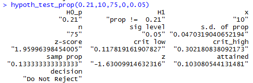
The displayed values include the standard deviation
of sample proportions and the z-score that we found in Figure 1,
the low and high critical values that we found in Figure 2,
the sample proportion that we found in Figure 3, and the attained
significance that we found in Figure 4.
Figure 10 includes the decision to not reject
H0.
The second static example had a sample size of 45, 14 items had
the characterisitic, the null hypothesis held that the
true proportion is 0.25, the alternative hypothesis is
that the proportion is greater than 0.25, and we want a 0.0625
level of significance. Using all of that we form the command
hypoth_test_prop(0.25,14,45,1,0.0625)
the results of which are in Figure 11.
(Note that the fourth argument, 1, could be any positive number
to show that the alternative hypothesis is the "greater than" choice.)
Figure 11
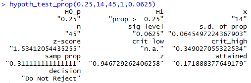
We see in Figure 11 values that we first
computed in
Figure 6 and Figure 7.
The third static example had a sample size of 35, 21 items had
the characterisitic, the null hypothesis held that the
true proportion is 0.7, the alternative hypothesis is
that the proportion is less than 0.7, and we want a 0.03
level of significance. Using all of that we form the command
hypoth_test_prop(0.7,21,35,-1,0.03)
the results of which are in Figure 12.
(Note that the fourth argument, -1, could be any negative number
to show that the alternative hypothesis is the "less than" choice.)
Figure 12
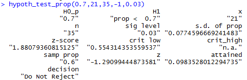
We see in Figure 12 values that we first
computed in
Figure 8 and Figure 9.
Below is a listing of the R
commands used in generating this page.
source("../gnrnd4.R")
source("../make_freq_table.R")
75*0.21
75*(1-0.21)
75/4000
sqrt(0.21*(1-0.21)/75)
qnorm(0.025)
qnorm(0.025,lower.tail=FALSE)
sigma <- sqrt(0.21*(1-0.21)/75)
z_left <- qnorm(0.025)
z_right <- qnorm(0.025,lower.tail=FALSE)
crit_low <-0.21 + z_left*sigma
crit_high <- 0.21 + z_right * sigma
crit_low
crit_high

gnrnd4(623127407,6997566)
L1
table(L1)
make_freq_table(L1)

sigma <- sqrt(0.21*(1-0.21)/75)
z <- (10/75-0.21)/sigma
# since the proportion is lower than 0.21
# look at the left tail
prob <- pnorm(z)
prob
prob*2


sigma <- sqrt(0.21*(1-0.21)/75)
z_left <- qnorm(0.0625)
z_right <- qnorm(0.0625,lower.tail=FALSE)
crit_low <-0.21 + z_left*sigma
crit_high <- 0.21 + z_right * sigma
crit_low
crit_high


sigma <- sqrt(0.25*(1-0.25)/45)
sigma
z_right <- qnorm(0.0625,lower.tail=FALSE)
crit_high <- 0.25 + z_right * sigma
crit_high

p_hat <- 0.3111
sigma <- sqrt(0.25*(1-0.25)/45)
sigma
z <- (p_hat-0.25)/sigma
z
prob <- pnorm(z, lower.tail=FALSE)
prob

0.7*35
(1-0.7)*35
0.05*7589
sigma <- sqrt(0.7*(1-0.7)/35)
sigma
z_left <- qnorm(0.03)
z_left
crit_low <- 0.7 + z_left * sigma
crit_low

p_hat <- 0.6
sigma <- sqrt(0.7*(1-0.7)/35)
sigma
z <- (p_hat-0.7)/sigma
z
prob <- pnorm(z)
prob

source( "../hypo_prop.R")
hypoth_test_prop(0.21,10,75,0,0.05)
hypoth_test_prop(0.25,14,45,1,0.0625)
hypoth_test_prop(0.7,21,35,-1,0.03)
Return to Topics page
©Roger M. Palay
Saline, MI 48176 February, 2016