GNRND5 -- Generate Random Samples 5 Version 1.0

This page describes the use and usefulness of both a program called "GNRND5", versions of which exist in Javascript and in R. This program goes beyond the earlier version, gnrnd4, which was limited by virtue of its needing to run on the Texas Instrunments graphing calculators, those in the TI=83/84 family. Unfortunately, gnrnd4 and gnrnd5 are not compatible.

It is fairly easy to use the functionality of gnrnd5 in web pages to create random sets of values that students can then generate in an R session. In that way the students can practice various statistical processes with randomly generated data sets determined by the web page and processed by other Javascript routines to create the results that the students should find by using R.

We communicate the desired settings for the R program by specifying two or three key values. These include the desired\sample size, the style of the numbers to be generated, the random seed value needed to generate the same numbers as are in the web page, and the other essential parameters for the generation.

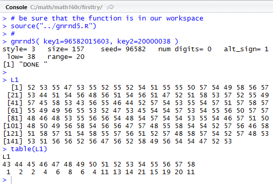
For example, this page generates the following table, based on the seed value 96582, showing holds 157 integer values which approximate a skewed left distribution with values ranging from about 38 to 58. However, using R we could generate the same values into a vector called L1 (this is the standard place that gnrnd5 creates the values) and and then display those values as shown in Figure 1.

Figure 1

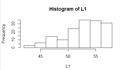
Note that the values in Figure 1 are identical to those in Table 1 above. Also, in Figure 1 we see the result of the of the table(L1) command showing the frequency of each value in the vector. This confirms the "left-skewed" distribution. To see more evidence of this distribution we could use the simple hist(L1) command to produce Figure 2.

Figure 2

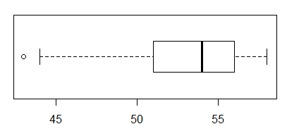
or the simple boxplot(L1,horizontal=TRUE) command to produce Figure 3.

Figure 3

At the end of this page there are formal definitions of the various parametric values that one feeds to gnrnd5 in order to achieve various results. At this time there are 10 different styles of generated data;

Uniform -- a uniform distribution from a given low value across a given range of values;
Power -- a skewed right distribution from a given low value across a given range of values;
Root -- a skewed left distribution from a given low value across a given range of values;
Normal -- a approximatly normal distribution aimed at having a given mean and standard deviation;
Bi-modal -- actually two overlapping normal distributions
Linear Regression -- paired values that conform, to a given degree, to a linear model given as the slope and intercept of the desired model;
Discrete -- a distribution of discrete values from 1 to the given number of different values having an approximation to specified relative frequencies;
Table -- Unlike other styles, this one creates a matrix of values based upon given goals for row and column relative frequencies;
Quartile -- a distribution that tries to conform to given percentages for the four quartiles with values from a given low scross a given range;
Paired Normal -- generates an approximately normal set of values with a given target mean and standard deviation, along with a second set of values that, to a specified extent, approximate the original set of values.

Before we get to the formal definitions here are some examples of each of the styles.

Uniform Example

A uniform distribution spreads values across some range where we expect that, for a a large sample size, we would have the values evenly spread across that range. For example, the values shown in Table 2 are all between 74 and 90 inclusive. There are only 180 such values but they cover the range with a fairly even distribution.

Power Example

A power distribution spreads values across some range where we expect that, for a a large sample size, we would have more of the values in the lower half of that range. For example, the values shown in Table 4 are all between 22 and 38 inclusive. There are only 215 such values but they cover the range with a more of the values in the lower half of the range.

Root Example

A root distribution spreads values across some range where we expect that, for a a large sample size, we would have more of the values in the upper half of that range. For example, the values shown in Table 6 are all between 41 and 57 inclusive. There are only 222 such values but they cover the range with a more of the values in the upper half of the range.

Normal Example

A normal distribution should spread its values about its mean with the usual bell shaped distribution. That is, we expect to find about 34% of the values between the mean and 1 standard deviation below the mean, with another 34% of the values between the mean and 1 standard deviation above the mean. About 95% of all the values should be between 2 standard deviations belpow and 2 standard deviations above the mean. Of course, in any sample the actual distribution will merely approximate that kind of spread. For us, we need to specify the goal mean and the goal standard deviation. For example, the values shown in Table 8 are generated where the goal mean is 17.4 and the goal standard deviation is 5.2 with values expressed to the nearewst tenth.

Bi-modal Example

For a bi-modal sample we merely need to specify two normal populations with different means. In general it is helpful to have the two populations have about the same standard deviation but this is not at all a requirement. It is also helpful to have the two means at least two standard deviations apart. We need to specify the goal mean and the goal standard deviation of one population (in key 2) and the goal mean and goal standard deviation of the other population (in key 3). For example, the values shown in Table 10 are generated where one goal mean is 45.1 with a standard deviation of 5.2 and the other goal mean is 22.8 with a standard deviation of 5.8 with values expressed to the nearewst tenth.

Linear Example

This style generates pairs of values, (x,y), such that these points approximate a line specified by dy=mx+b. We specify the equation in this way so that d, m, and b can be integer values. The degree of approximation is set by yet another parameter, one given in key 2. To do this we specify the Low value for the x-values and a Range for the x-values.

Thus to generate points close to the line y=(4/3)x+9/4, first we convert that equation to 12y=16x+27. Then, we specify the lowest possible x value amd the range of the x values; for this example we will generate values between 5.7 and 18.6, all with at most two decimal places. Finally, by choosing a small "error factor", say 3, we will get points that are fairly close to the specified line.

The R script
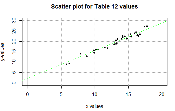
source("../gnrnd5.R") gnrnd5( key1=260561003006, key2=3120027016012, key3=1290000570 ) plot(L1,L2, xlab="x-values", ylab="y-values", main="Scatter plot for Table 12 values", xlim=c(0,20), ylim=c(0,30), pch=20 ) abline(h=0,v=0) abline(h=seq(5,30,5),lty="dotted", col="darkgray") abline(v=seq(5,20,5),lty="dotted", col="darkgray") abline(9/4, 4/3, col="green", lty="dashed")
produced the following plot in Figure 4. Note that the goal relationship is shown as a dashed green line in the plot. That is the goal relationship not the linear regression line.

Figure 4

Discrete Example

A discrete distribution generates values from 1 through the given number of categories in the approximate relative frequencies specified for those categories. For example, the values shown in Table 13 are all integers 1, 2, 3, 4, and 5. The aim is to have the respective relative freuencies of 10% for 1's, 40% for 2's, 5% for 3's, 15% for 4's, and 30% for 5's. Of course, with just 319 values we will get an approximation to that distribution.

Table Example

This style generates not a vector of values but rather a contingency table of values. That is, we need to specify the number of rows and the number of columns in the table. Then we specify the relative row frequency and the relative column frequency. With that information in hand, the program generates and records values that fall into row and a column according to the relative frequencies and the program then tallies in the appropriate row and column of the table the fact that such a value was generated. In a perfect world the resulting matrix would demonstrate an independence between row and column characteristics. Of course, with smallish sample sizes the resulting table may be a bit off from that independence.

We want to be able to encourage the deviation from independence. To do this the program inappropriately uses the value of the number or decimal digits divided by 45 as a cutpoint for forcing a choice in a preselected random row to go into a preselected random column. If the number of digits to be used is 0 then there is no encouraging change to the random distriution of values according to the specified row and column proportions.

For example, here is a table created with row proportions 9:2:7:5 and column proportions 2:7:9:3:8, with a size specification of 143 and with 0 as the number of digits. Then, here we generate the same table, but this time with the number of digits set to 8.

Quartile Example

A quartile distribution allows the user to specify the span of the quartiles across a range of values. Thus, we might want values from a low of 13.2 to a high of 97.2 but we might want the first 25% of those values between 13.2 and 54.1, the second quartile of values between 54.1 and 58.4, the third quartile between 58.4 and 68.8, and the last quartile of values between 68.8 and 97.2. Thus we have a range of 84.0 and the first quartile has a span of 40.9, thus it covers about 49% of the range. The second quartile has a span of 4.3 which is about 5% of the range. The third quartile has a span of 10.4 or about 12% of the range, leaving about 34% of the range for the fourth quartile. Table 15 has a data set that approximates that description.

Paired Normal Example

The paired normal distribution generates values that are approximately normally distributed with a specified mean and a specified standard deviation. In addition, the program generates a second list with values paired to the first list. This would be especially useful in looking at situations where we are looking at the mean of the differences of paired values.

For example, consider the Pre-event data that is normal with mean 37.6 and standard deviation of 7.3, along with the paired Post-event data that is a bit different from the first values. Table 16 has a data set that approximates that description.

Formal Description of Parameters for GNRND5

Key 1	d	d d d d d	d d d d	d d
	num digits	initial seed value	(generated sample size)-1	style
	Number of decimal digits implied in some second key values and used in generating the actual values in some cases. Also used to determine if certain second key values are negative. Values 0, 1, 2, 3, and 4 represent, respectively 0, 1, 2, 3, or 4 decimal digits. Values 5, 6, 7, 8, 9 represent, respectively, 0, 1, 2, 3, or 4 decimal digits, but with the understanding that some second key values may be negative.	The initial seed value. Generally this is determined by some other random number generator. The value used here then determines the sequence of random values generated by the appropriate functions both in the TI-83/84 program and in the web page.	One less than the desired sample size. Thus a 4-tuple of digits such as 0311 will generate a 312 item sample, a 4-tuple of digits such as 9932 will generate a 9933 item sample, and a 4-tuple of digits such as 0003 will generate a 4 item sample.	The style selector. This gives us room for up to 99 different styles of samples. Initially there are 10 defined styles, As more styles are specified this list will expand, Current styles are Uniform Power Root Normal Bi-modal (mixed normal) Linear Regression Discrete Frequency table Quartile points Paired Normal In general, the particular style chosen determines the meaning of the second key.

Style	Name	Text
01:	Uniform	A uniform distribution gives an equally likely probability of having each permissible greater than or equal to some specified Low value and a High value determined to be the Low+Range for some specified Range, This is accomplished by taking a uniformly distributed random value between 0 and 1 and applying it to the Range, adding the result to the Low value, and then rounding the result to the specified number of digits.
02:	Power	This power distribution is identical to the uniform distribution except that the random value that is generated is squared before it is used to scale the Range. The result, since the random values generated initially are between 0 and 1, is to have a distribution that favors low values.
03:	Root	This power distribution is identical to the uniform distribution except that we take the quare root of the random value that is initially generated before it is used to scale the Range. The result, since the random values generated initially are between 0 and 1, is to have a distribution that favors high values.
Key 2	d d d d d d		d d d d d d
	These six digits specify the Range of values that may be generated. Note that the number of decimal digits specified in Key 1 places an implied decimal point within the specified digits. Thus, the value 000100 (which could be specified simply as 100) would mean, 100 if the number of decimal digits in Key 1 is 0 or 5. On the other hand, 100 would mean 0.100 if the number of decimal digits in Key 1 is 3 or 7.		These six digits represent the Low end of the permisible values to be generated. Note that if the number of digits specied in Key 1 came from a value greater than 4 then this Low values is set to be a negative, Thus, 120000 with the number of decimal digits given as a 6, has an implied decimal value of 1200.00, but it is a negative value, that is, -1200.00.

Style	Name	Text
04:	Normal	The program generates values that are approximately normally distributed with a specified mean and a specified standard deviation.
Key 2	d d d d d d		d d d d d d
	These six digits specify the goal Standard Deviation of values to be generated. Note that the number of decimal digits specified in Key 1 places an implied decimal point within the specified digits. Thus, the value 000100 (which could be specified simply as 100) would mean, 100 if the number of decimal digits in Key 1 is 0 or 5. On the other hand, 100 would mean 0.100 if the number of decimal digits in Key 1 is 3 or 7.		These six digits specify the goal Mean of values to be generated. Note that if the number of digits specied in Key 1 came from a value greater than 4 then this Mean values is set to be a negative, Thus, 020000 with the number of decimal digits given as a 6, has an implied decimal value of 200.00, but it is a negative value, that is, -200.00.

Style	Name	Text
05:	Bi-Modal	The program generates values that are randomly selected from two approximately normal distributions, each with its own specified mean and standard deviation. Key 2 will give the mean and standard deviation for one distribution, while Key 3 will give the mean and standard deviation for the other distribution. As it generated each value, the process randomly selects which distribution to use. As such, the number of values from each distribution is a random choice and there is no attempt to have an approximately equal number of values from each distribution.
Key 2	d d d d d d		d d d d d d
	These six digits specify the first goal Standard Deviation of values to be generated. Note that the number of decimal digits specified in Key 1 places an implied decimal point within the specified digits. Thus, the value 000100 (which could be specified simply as 100) would mean, 100 if the number of decimal digits in Key 1 is 0 or 5. On the other hand, 100 would mean 0.100 if the number of decimal digits in Key 1 is 3 or 7.		These six digits specify the first goal Mean of values to be generated. Note that if the number of digits specied in Key 1 came from a value greater than 4 then this Mean values is set to be a negative, Thus, 320000 with the number of decimal digits given as a 6, has an implied decimal value of 3200.00, but it is a negative value, that is, -3200.00.
Key 3	(-) d d d d d d		d d d d d d
	These six digits specify the goal Standard Deviation of values to be generated. Note that the number of decimal digits specified in Key 1 places an implied decimal point within the specified digits. Thus, the value 000100 (which could be specified simply as 100) would mean, 100 if the number of decimal digits in Key 1 is 0 or 5. On the other hand, 100 would mean 0.100 if the number of decimal digits in Key 1 is 3 or 7. The negative sign, if present has no effect on the standard deviation, rather, if there is a leading negative sign then the value of the mean, the last six digits, is made negative.		These six digits specify the second goal Mean of values to be generated. Note that, unlike the first goal mean, this one is turned negative by preceding the entired specified key value with a negative sign.

Style	Name	Text
06:	Linear	The linear distribution generates pairs of values, (x,y), such that there is a y=mx+b underlying relationship between the values. To generate our distribution we need to have a Low value for the x-values, a Range for the x-values, a specification for the linear relationship, given as Dy =Mx+B, and an indicator for the maximum amount of error to introduce. The Low and Range values are given in Key 3 while the other valeus are specified in Key 2.
Key 2	d	d	d	d d d d	d d d	d d d
	This is a single digit error factor. To calculate the maximum allowed error on any one observation, if E is this digit, find (E+1)(E+2)/200 and apply that to the max change in the model from the Left x value to the Right x value.	This digit indicates the sign of the B value: 0-5=positive; 6-9=negative.	This digit indicates the sign of the M value: 0-5=positive; 6-9=negative.	These four digits give the value of B in Dy=Mx+B, possibly negated from earlier indicator.	These three digits give the value of M in Dy=Mx+B, possibly negated from earlier indicator.	These three digits give the value of D in Dy=Mx+B.
Key 3	d d d d d d			d d d d d d
	These 6 digits give the Range of the x-values. Note that this value is scaled by the number of decimal digits specified in Key 1.			These 6 digits give the Low value of the x-values. Note that this value is scaled by the number of decimal digits specified in Key 1. In addition, this value may be changed to a negative value based on that same Key 1 value.

Style	Name	Text
07:	Discrete		The discrete distribution generates values from 1 to the number of categories in an approximation to the relative frequency given for each of the categories. There should be at least two categories and there can be as many as nine categories. The number of categories and the relative frequencies, as single digits, for each category are given in Key 2.
Key 2	d	d	d	d	d	d	d	d	d	d
Key 2	Relative Freq cat 9	Relative Freq cat 8	Relative Freq cat 7	Relative Freq cat 6	Relative Freq cat 5	Relative Freq cat 4	Relative Freq cat 3	Relative Freq cat 2	Relative Freq cat 1	# of cat

Style	Name	Text
08:	Table		The Table distribution fills a table with the number of times a value has been observed in each cell of the table. This is done with a goal of having a certain relative frequency in each row and certain relative frequency in each column of the table. The second Key gives the number of rows and the number of columns, along with a relative frequency of each. The specification below for that second key implies that the sum of the number of rows and number of columns should not excede eight (8). In fact, it can be 14. A further note is that the actual number of "observations" is equal to the "size" as given in Key 1 times the number of rows times the number of columns. This is done because having so many cells in a table means that the "observations" are spread out over many cells. Using this factor approach allows us to get much larger values.
Key 2	d	d	d	d	d	d	d	d	d	d
	Relative Freq col n	Relative Freq col n-1	Relative Freq col n-2	Relative Freq	Relative Freq	Relative Freq	Relative Freq row 2	Relative Freq row 1	# of cols	# of rows
	As implied above, these 8 digits hold the relative frequencies of the rows and columns. Reading right to left we find the relative frequency of row 1, row 2, and so on until we are done with the row values. Then we start with the column relative frequencies. Since there are but 8 digits in this group, we want the number of rows plus the number of columns to be no more than 8. The actual limit is 14, but the documentation here is a bit easier if we show only 8.

Style	Name	Text
09:	Quartile	The Quartile Points distribution chooses random values from the Low value to the Low+Range value such that we have Quartile points set at a specified percent across the range of values. Thus, we could have a range of 300 and specify quartile widths (i.e., the span) at 50%, 15%, 25%, and 10%. These correspond to a span of 150, 45, 75, and 30. The range of values is divided accordingly. Quartile points are set, remaining values are allocated. The values are placed in the list in random order. Also, If the IQR is such that 1.5*IQR does not cover the first or fourth quartile, then the program ensures that there is one point in the outlier region. Finally, the specified size for the sample is always rounded up to one less than the next multiple of 4.
Key 2	pp	pp	pp	d d d d	d d d d
Key 2	This is the percent of the range given to the first quartile.	This is the percent of the range given to the second quartile.	This is the percent of the range given to the third quartile. Note that the fourth quartile gets the remaining part of the range.	These four digits give the range, possibly altered by the number of decimal digits.	These four digits give the low value, possibly altered by the number of decimal digits.

Style	Name	Text
10:	Paired Normal	The program generates values that are approximately normally distributed with a specified mean and a specified standard deviation. In addition, the program generates a second list with values paired to the first list.
Key 2	d d		d d d d d d	d d d d d d
Key 2	These two digits specify the spread of the paired values. In particular, values near 00 produce almost no spread while values near 99 produce a great spread and one that is shifted to have the second value tending to be greater than the first.		These six digits specify the goal Standard Deviation of values to be generated. Note that the number of decimal digits specified in Key 1 places an implied decimal point within the specified digits. Thus, the value 000100 would mean, 100 if the number of decimal digits in Key 1 is 0 or 5. On the other hand, 000100 would mean 0.100 if the number of decimal digits in Key 1 is 3 or 8.	These six digits specify the goal Mean of values to be generated. Note that if the number of digits specied in Key 1 came from a value greater than 4 then this Mean values is set to be a negative, Thus, 020000 with the number of decimal digits given as a 7, has an implied decimal value of 200.00, but it is a negative value, that is, -200.00.