GNRND4 -- Generate Random Samples 4 Version 1.2

This page describes the use and usefulness of both a TI-83/84 program called "GNRND4", the similar R script "gnrnd4.R", and an associated Javascript routine called "gnrnd4()".

This page has three sections:

Why do this? The background: to explain the need for such programs.
Examples of the various kinds of values that gnrnd4 can generate.
Formal description of key values for generating different sets of values.

Why do this? The background:

The Texas Instrunments graphing calculators are capable of producing random values. In particular, this includes the TI-83, the TI-83Plus, and the TI-84Plus. It is fairly easy to use that functionality to create random sets of values that students can use to practice various statistical processes. By setting an initial SEED value for the random number generator, each student's calculator will generate the same sequence of pseudo-random values. Therefore, we could easily write a program for the calculator to generate 20 values that are

uniformly distributed by using the rand function,
integers between given bounds using the randInt function,
the result of a binomial experiment using the randBin function, or
normally distributed with a given mean and standard deviation using the randNorm function.

Javascript, a language behind many features on web pages, can also generate random values. These can be displayed on web pages, be they pages that provide examples, pages that demonstrate certain computations or descriptive techniques, or even pages that are tests for students to take. Thus, using javascript, it is easy to generate on a web page a table of some size holding random values within some range. For example, the table below holds between 45 and 60 values, each randomly generated to be between 20 and 80.

The table above holds random numbers that are uniformly distributed between 20 and 80. Each time this page is loaded or refreshed, the size of the table and the numbers in the table are regenerated. With only a bit more programming, we could change the Javascript behind that table so that it produces a set of integers that is approximately normally distributed with a given mean and standard deviation. The following table holds just such a set of values.
With similar modifications we could produce other distributions for a table on the web.

What we have seen is that we can produce random sets of values on the TI-833/84 calculators and on web pages via Javascript. Needless to say, we can produce random values in R. The real problem is that if we generate a random set of values on a web page we want to be able to generate the same set of valuse on the TI-83/84 calculator or in an R session. What we do not want to do is to ask students to enter all of the numbers by hand. For any sizable set of values, say more than 15, the odds of doing so correctly are small. The time required is significant. The learning achieved by entering data is minimal at best. All of this gives rise to the GNRND4 system. Using this system we can produce a table of values on the web and give students two, or sometimes three, key values to enter into the GNRDN4 program on their calcualtor or into their R-script. The GNRND4 program will then generate the same set of values that we on the web page within the calculator or in the R session, completely saving the sudents from having to enter a long list of values.

Examples

Here are eamples of the various kinds of values that we can produce using GNRND4 on the TI-83/84 calculator, or using gnrnd4() in an R script.

Uniform distribution
Power distribution
Root distribution
Normal distribution
Bi-modal distribution
Linearly related distributions
Discrete distribution
Contingency Table -- first methodology
Quartile distribution
Paired Normal distributions
Contingency Table -- second methodology

Uniform Example

As an example we will generate a sequence of uniformly distributed values with 1 decimal digit, values between -100 and 100, with 35 values. Here is such a data set.

Here is the text of an R script that would produce these same values in a variable called L1, and then display those values and compute some descriptive statistics for those values.

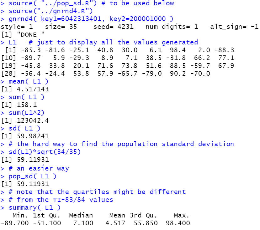
source( "../pop_sd.R") # to be used below
source("../gnrnd4.R")
gnrnd4( key1=6042313401, key2=200001000 )
L1   # just to display all the values generated
mean( L1 )
sum( L1 )
sum(L1^2)
sd( L1 )
# the hard way to find the population standard deviation
sd(L1)*sqrt(34/35)  
# an easier way
pop_sd( L1 )
# note that the quartiles might be different
# from the TI-83/84 values
summary( L1 )

Here is the R console output from the above commands:

On the TI-83/84 calculator we can run the GNRND4 program with a the first key value as 6042313401 and the second key value as 200001000. This will produce a list in L₁ on the calculator. The following screen images were taken from just such an run of the GNRND4 program on a TI-84.

Figure 1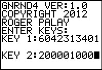	Figure 2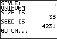	Figure 3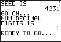
Figure 4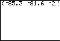	Figure 5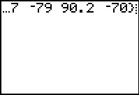	Figure 6 From STAT EDIT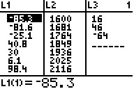
Figure 7 From 1-Var Stats	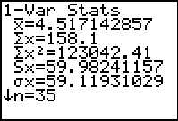Figure 8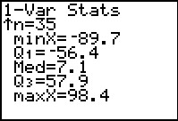

In particular, we can see the KEY values being entered in Figure 1 and the list of values shown in Figures 4 and 5 from within the program, and again, the start of the list as shown in the DATA EDITOR in Figure 6. Figures 7 and 8 are provided to demonstrate that we can work with the data that has been placed in L₁. Again, note that the quartile values on the TI-83/84 use a different algorith than is used in R.

Comparing the values in the table with those shown in the Figures above, we see that gnrnd4() in R and the GRNRD4 program on the calculator produce the same values as we have produced on this web page.

Power Example

We will generate a sequence of skewed left values with 2 decimal digit, values between -10 and 10, with 38 values. Here is such a data set.

Here is the text of an R script that would produce these same values in a variable called L1, and then display those values.

# Generate a skewed left set of values
# this assumes we have loaded gnrnd4() into our environment
gnrnd4( key1=7042313702, key2=200001000 )
L1   # just to display all the values generated

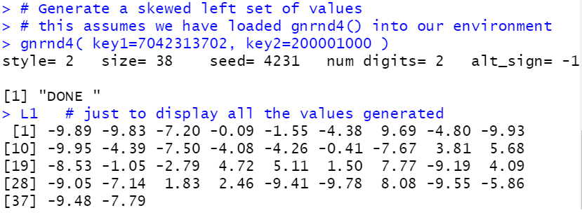
Here is the R console output from the above commands:

On the TI-83/84 calculator we can run the GNRND4 program with a the first key To generate a sequence of power distributed values (skewed left) with 2 decimal digit, values between -10 and 10, with 38 values, we can run the GNRND4 program on the calculator with a the first key values as 7042313702 and the second key value as 200001000. This will produce a list in L₁ on the calculator. The following screen images were taken from just such an run of the GNRND4 program on a TI-84.

Figure 9	Figure 10	Figure 11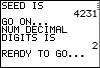
Figure 12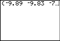	Figure 13 From STAT EDIT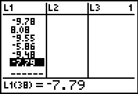

Comparing the values in the table with those shown in the Figures above, we see that gnrnd4() in R and the GRNRD4 program on the calculator produce the same values as we have produced on this web page.

Root Example

Next, generate a sequence of root distributed values, skewed right, with 0 decimal digits, values between 100 and 300, and with 27 values. Here is such a data set.

Here is the text of an R script that would produce these same values in a variable called L1, then display those values, and then compute some descriptive measures of that data.

# Generate a skewed right set of values
# this assumes we have loaded pop_sd() into our environment
# this assumes we have loaded gnrnd4() into our environment
gnrnd4( key1=042312603, key2=20000100 )
L1   # just to display all the values generated
mean( L1 ) # to find the mean
sum( L1 )  # to find the sum of the values in L1
           # to find the sum of the squares
sum( L1^2 )           #   of the values in L1
           # to find the standard deviation
sd( L1 )           #   if this is a sample
           # to find the standard deviation
pop_sd(L1)           #   if this is a population
summary(L1)# finds lots of values

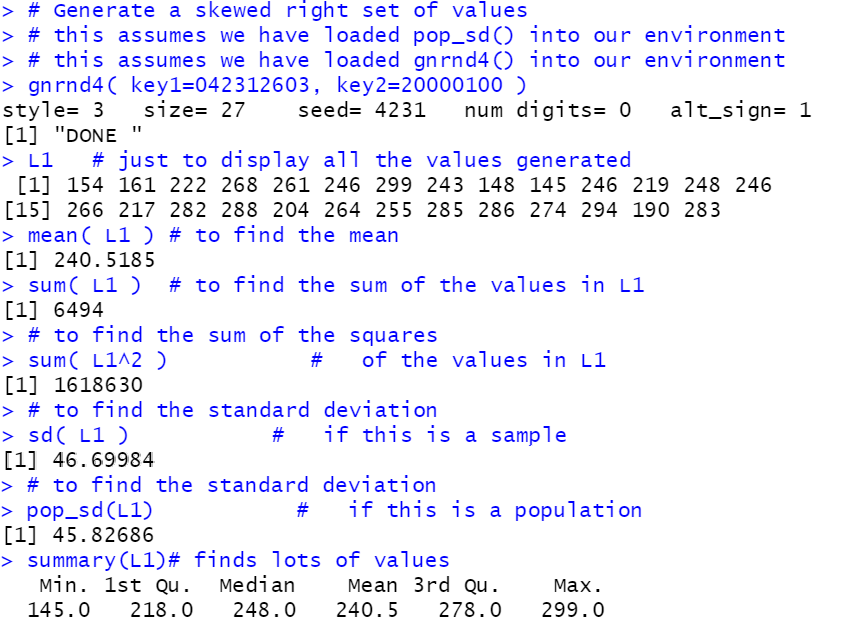
Here is the R console output from the above commands:

We can run the GNRND4 program on the calculator with a the first key values as 42312603 and the second key value as 20000100. This will produce a list in L₁ on the calculator. The following screen images were taken from just such an run of the GNRND4 program on a TI-84.

Figure 14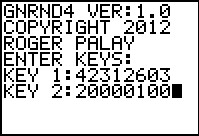	Figure 15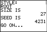	Figure 16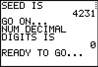
Figure 17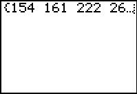	Figure 18 From STAT EDIT	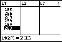Figure 19 From 1-Var Stats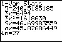
Figure 20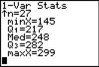

Comparing the values in the table with those shown in the Figures above, we see that gnrnd4() in R and the GRNRD4 program on the calculator produce the same values in our list of values as we have produced on this web page. We again note that R and the TI-83/84 calculator use slightly different algorithms for finding the first and third quartile. Both algorithms are accepted methodologies, and in fact there is a third accepted method that may produce yet other values.

Normal Example

Generate a sequence of approximately normally distributed values with 3 decimal digits, with an approximate mean = 10 and an approximate standard deviation = 3.2, with 45 values, Here is such a data set.

Here is the text of an R script that would produce these same values in a variable called L1, then display those values, and then compute some descriptive measures of that data.

# Generate an approximately normal set of values
# this assumes we have loaded pop_sd() into our environment
# this assumes we have loaded gnrnd4() into our environment
gnrnd4( key1=3042314404, key2=0320010000 )
L1   # just to display all the values generated
mean( L1 ) # to find the mean
sum( L1 )  # to find the sum of the values in L1
           # to find the sum of the squares
sum( L1^2 )           #   of the values in L1
           # to find the standard deviation
sd( L1 )           #   if this is a sample
           # to find the standard deviation
pop_sd(L1)           #   if this is a population
summary(L1)# finds lots of values

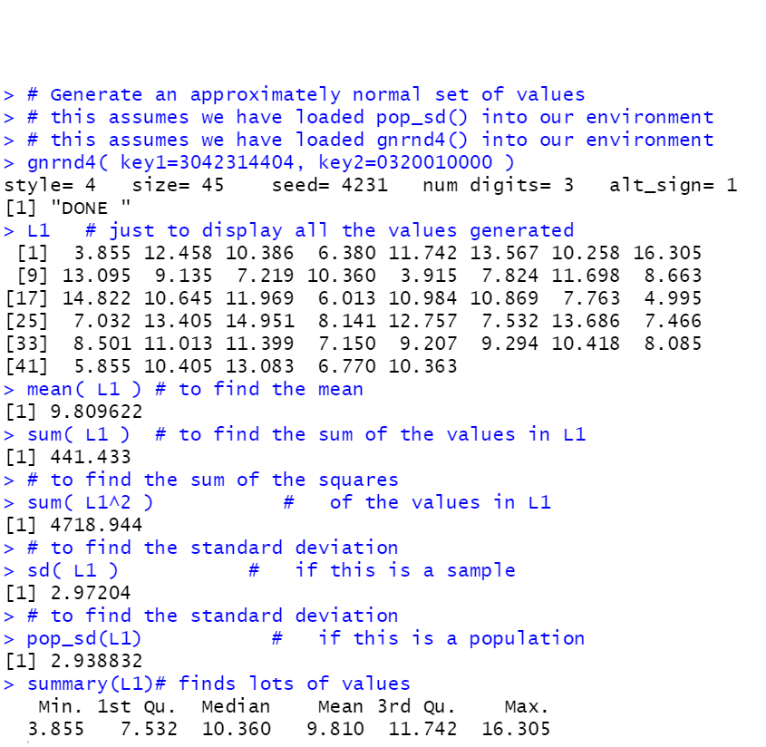
Here is the R console output from the above commands:

We can run the GNRND4 program on the calculator with a the first key values as 3042314404 and the second key value as 320010000. This will produce a list in L₁ on the calculator. The following screen images were taken from just such an run of the GNRND4 program on a TI-84.

Figure 21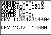	Figure 22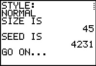	Figure 23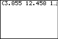
Figure 24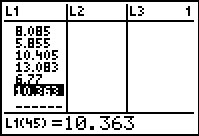	Figure 25 From 1-Var Stats	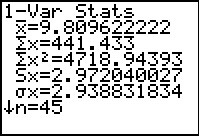Figure 26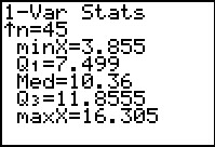

Bi-Modal Example

Generate a sequence of bi-modally distributed values, built from two approximately normal distributions, with 1 decimal digits, built from distributions that are N(30,10) and N(40,5) with a total of 54 values. Here is such a data set.

Here is the text of an R script that would produce these same values in a variable called L1, then display those values, and then compute some descriptive measures of that data.

# Generate an approximately bimodal set of values
# this assumes we have loaded pop_sd() into our environment
# this assumes we have loaded gnrnd4() into our environment
gnrnd4( key1=1042315305, key2=10000300, key3=5000400 )
L1   # just to display all the values generated
mean( L1 ) # to find the mean
sum( L1 )  # to find the sum of the values in L1
           # to find the sum of the squares
sum( L1^2 )           #   of the values in L1
           # to find the standard deviation
sd( L1 )           #   if this is a sample
           # to find the standard deviation
pop_sd(L1)           #   if this is a population
summary(L1)# finds lots of values

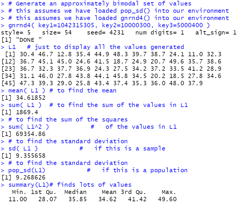
Here is the R console output from the above commands:

We can run the GNRND4 program on the calculator with a the first key values as 1042315305, a second key value as 10000300, and a third key as 05000400. This will produce a list in L₁ on the calculator. The following screen images were taken from just such an run of the GNRND4 program on a TI-84.

Figure 27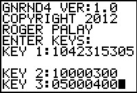	Figure 28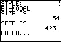	Figure 29
Figure 30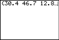	Figure 31 From STAT EDIT	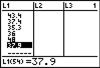Figure 32 From 1-Var Stats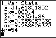

Linear Model

We want to generate a sequence of pairs of values, x and y, and we want these to be linearly related values with some component of an error. Do this for 19 pairs of values where the x values are between 10 and 30, where the model is y=(5/3)x+(4/3), with values having 1 decimal place and an error of about 10%. Here is such a data set.

Here is the text of an R script that would produce these same values in a variable called L1, then display those values, and then compute some descriptive measures of that data.

# Generate a set of pairs of values that have
#    an approximately linear relation.
# this assumes we have loaded pop_sd() into our environment
# this assumes we have loaded gnrnd4() into our environment
gnrnd4( key1=1042311806, key2=3120040503, key3=20000100 )
L1   # just to display all the x values generated
L2   # just to display all the y values generated
lm(L2~L1) # to show the coefficients in y=a + b*x
cor( L1,L2)   # the correlation coefficient, r
cor(L1,L2)^2  # the value of r^2
plot(L1,L2)   # a scatter plot

Here is the R console output from the above commands:

Here is the plot from the above commands:

We can run the GNRND4 program on the calculator with a the first key values as 1042311806, the second key value as 3110040503, and the third key as 0020000100. This will produce a list of x values in L₁ and a list of the corresponding y values in L₂ on the calculator. The following screen images were taken from just such an run of the GNRND4 program on a TI-84.

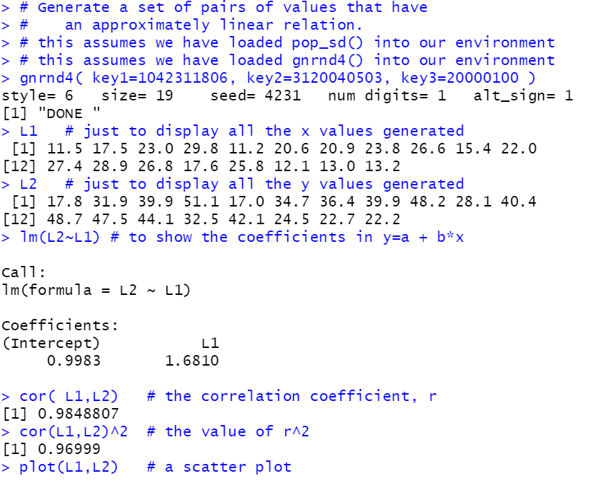
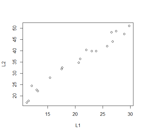
Figure 33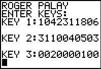	Figure 34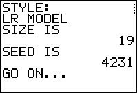	Figure 35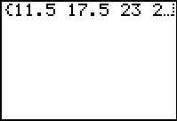
Figure 36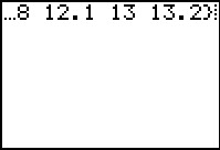	Figure 37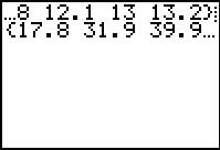	Figure 38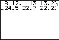
Figure 39 From STAT EDIT	Figure 40 From PLOT	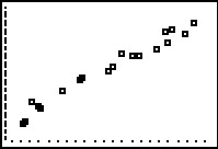Figure 41 From LinReg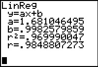

Discrete Example

Generate a sequence of discrete values that fall within just a small number of categories where we specify the number of categories and then the relative goal frequency for each such category. Thus, we might want to have 5 categories such that their goal relative frequency is given in the following table:

Frequency name	1	2	3	4	5
Relative frequency as a number	8	4	5	5	3
Relative frequency as a percent	32%	16%	20%	20%	12%

Here is such a data set.

Here is the text of an R script that would produce these same values in a variable called L1, then display those values, and then compute some descriptive measures of that data.

# Generate an approximately discrete set of values
#    corresponding to given relative frequencies
# this assumes we have loaded pop_sd() into our environment
# this assumes we have loaded gnrnd4() into our environment
gnrnd4( key1=042314207, key2=355485 )
L1   # just to display all the values generated
mean( L1 ) # to find the mean
# to find the standard deviation
sd( L1 )           #   if this is a sample
# to find the standard deviation
pop_sd(L1)           #   if this is a population
summary(L1)# finds lots of values
source("../make_freq_table.R")
make_freq_table( L1 )

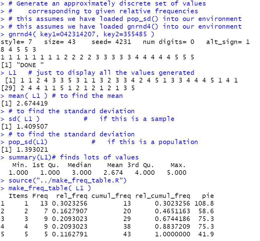
Here is the R console output from the above commands:

To create a distribution of 43 such values in L₁, we can run the GNRND4 program on the calculator with a the first key values as 42314207 and the second key value as 355485. This will produce a list in L₁ on the calculator. The following screen images were taken from just such an run of the GNRND4 program on a TI-84.

Figure 42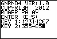	Figure 43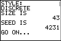	Figure 44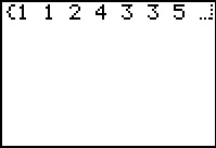
Figure 45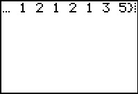	Figure 46 From STAT EDIT	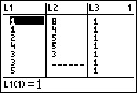Figure 47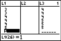
Figure 48 From COLLATE2	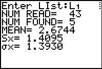Figure 49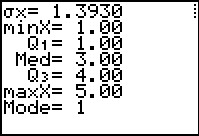	Figure 50 From STAT EDIT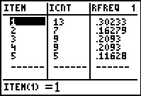

Table Example

Generate a contingency table of frequencies for just a small number of row and column. We specify the number of rows and the number of columns, and then the relative goal frequency for each row and of each column. Thus, we might want to have 3 rows and 5 columns such that their goal relative frequency is given in the following table:

	Col Name	1	2	3	4	5	Row Goal Freq
Row Name
1							7
2							4
3							5
	Column Goal Freq.	4	6	5	7	8

Note that the table above is not a frequency table of observations but rather it just gives the goal frequencies for the rows and columns. When we generate the actual frequency table we will aim to meet those row and column goal proportions. As such, the resulting table should approximate independence.

Here is such a data set.

Here is the text of an R script that would produce these same values in a variable called matrix_A, then display those values.

# Generate a contingency table that has approximate
# row and column distributions
gnrnd4( key1=042310908, key2=8756454753 )
matrix_A   # just to display all the values generated

Here is the R console output from the above commands:

To generate such a table in matrix [A], we can run the GNRND4 progam with a the first key values as 42310908 as the first Key value and the second key value as 8756454753. This will produce a table of 150 observations (10*number of rows*number of columns) distributed across 5 columns and 3 rows, with the approximate row and column goal frequencies as given above. [Notice that in this case the usual specification of "size" is used as a multiplier times the number of cells in the table. This is due to the fact that for a given tables size such as 3 by 5 with 15 cells, we may want way more than just 100 entries which would have been the normal limit for size.] The following screen images were taken from just such an run of the GNRND4 program on a TI-84.

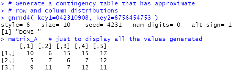
Figure 51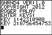	Figure 52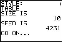	Figure 53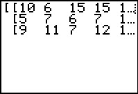
Figure 54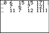

The same table is produced below with the row and column totals, and then the row and column percents appended to the table. The COLLATE3 program on the TI-83/84 and the collate3() function in R can produce this same data.

Quartile Example

The goal of the Quartile option is to specify a range of values and then to generate random values within that range such that Q₁, Q₂, and Q₃ occur at specified percentages of that range. Thus, we might want the quartile widths to be the following percent of the overall range:

Quartile name	Q1	Q2	Q3	Q4
Percent of range in quartile	50%	15%	25%	10%

Here is such a data set with 95 values in the range from 400 to 700 where Q₁ is at 50% of that range, i.e., at 550, Q₂ is 15% further in the range, i.e., at 595, and Q₃ is 25% further in the range, i.e., at 670.

Here is the text of an R script that would produce these same values in a variable called matrix_A, then display those values.

# Generate a distribution into a specified range such
# that quartiles happen at particular values in that
# range
gnrnd4( key1=042319409, key2=501525300400 )
L1   # just to display all the values generated
   #Now look at the quartiles, remembering that R uses a
   # different algorithm for calculating the quartiles
   # than does the TI-83/84 calculators.  Therefore, we
   # expect that the results here will be close to but
   # not exactly the same as the reported results from
   # the TI-83/84 calculators.
summary(L1) # to examine the quartiles

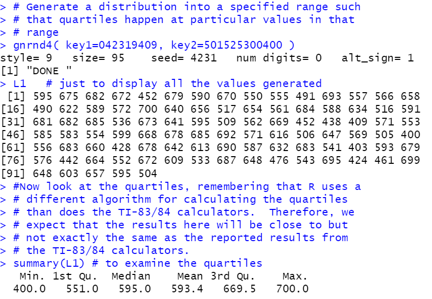
Here is the R console output from the above commands:

To create a distribution of 95 such values on a TI-83/84 calculator we run the GNRND4 program with a the first key values as 42319409 and the second key value as 501525300400. This will produce a list in L₁ on the calculator. The following screen images were taken from just such an run of the GNRND4 program on a TI-84.

Figure 55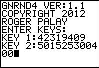	Figure 56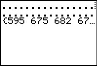	Figure 57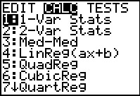
Figure 58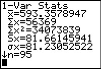	Figure 59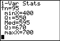	Figure 60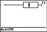

Paired Normal Example

Generate a sequence of normally distributed values with a given mean and standard deviation, and then produce a parallel set of values that deviate by a given extent of random deviation from the first set of values. Here is such a data set.

Here is the text of an R script that would produce these same values in two lists called L1 and L2, then display those values.

# Generate a normal distribution given mean and standard
# deviation and generate paired values with a given 
# the extent of random deviation from the first values.

gnrnd4( key1=1427372510, key2=110008500425 )
L1   # just to display all the x values generated
L1   # just to display all the y values generated
# look at the summary descriptions of both lists
source("../long_summary.R")
long_summary(L1)
long_summary(L2)
# find the differences
L3 <- L1 - L2
L3

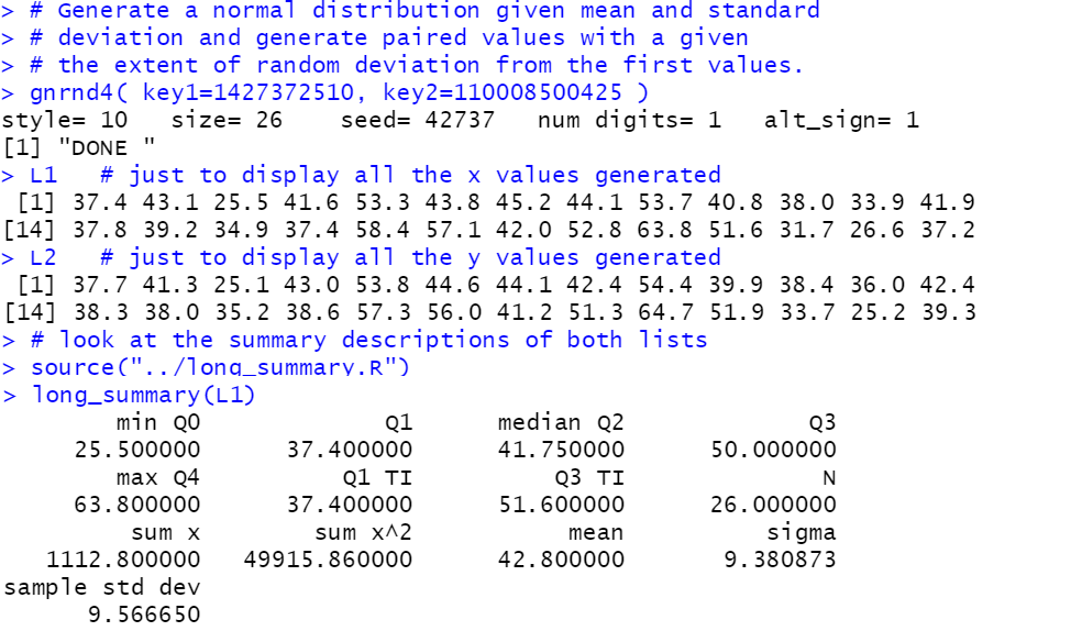
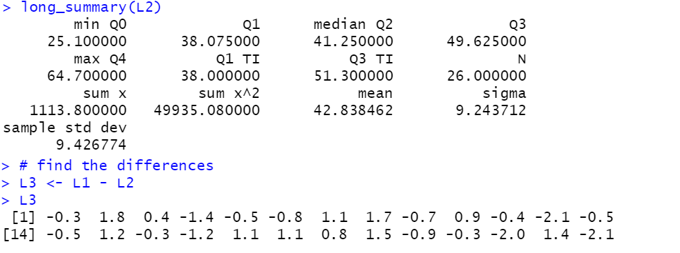
Here is the R console output from the above commands:

To get the same values with 1 decimal digit, with an approximate mean = 42.5 and an approximate standard deviation =8.5, with 26 values, we can run the GNRND4 program on the calculator with a the first key values as 1427372510 and the second key value as 110008500425. This will produce a list in L₁ on the calculator. It will also produce a list in L₂ that holds paired values where we can control, to some extent, the spread of the pairing. The following screen images were taken from just such an run of the GNRND4 program on a TI-84.

Figure 61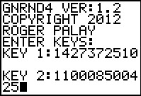	Figure 62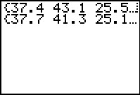	Figure 63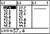
Figure 64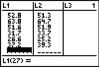	Figure 65 From 1-Var Stats for L1	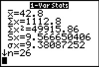Figure 66 From 1-Var Stats for L2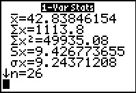
Figure 67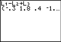	Figure 68	Figure 69

Independence Example

Whereas the earlier Table Example generated a contingency table that was in some ways approximately independent, here we generate a contingency table that will just fail a test for independency at a given level of significance.

This option has not been implemented in the TI-83/84 GNRND4 program. It only works for the R script gnrnd4().

	Col Name	1	2	3	4	5	Row Goal Freq
Row Name
1							7
2							4
3							5
	Column Goal Freq.	4	6	5	7	8

Note that the table above is not a frequency table of observations but rather it just gives the goal frequencies for the rows and columns. When we generate the actual frequency table we will have those row and column goal proportions. However, the details of the table will cause the test for independence to just fail at a given level.

Here is such a data set.

Here is the text of an R script that would produce these same values in a variable called matrix_A, then display those values.

# Generate a contingency table that has specific
# row and column distributions but that rejects 
# independence at the 0.10 level of significance.
gnrnd4( key1=042313911, key2=8756454753 )
matrix_A   # just to display all the values generated

source("../crosstab.R")
crosstab( matrix_A )    # to get the analysis of the matrix
totals  # to see all of the row and column totals
# a quick look at the expected values
# for perfect independence
expected
# the chi-squared value, with 8 degrees of freedom,
# that has 10% of the area under the curve to the
# right of this value
qchisq(0.10,8,lower.tail=FALSE)

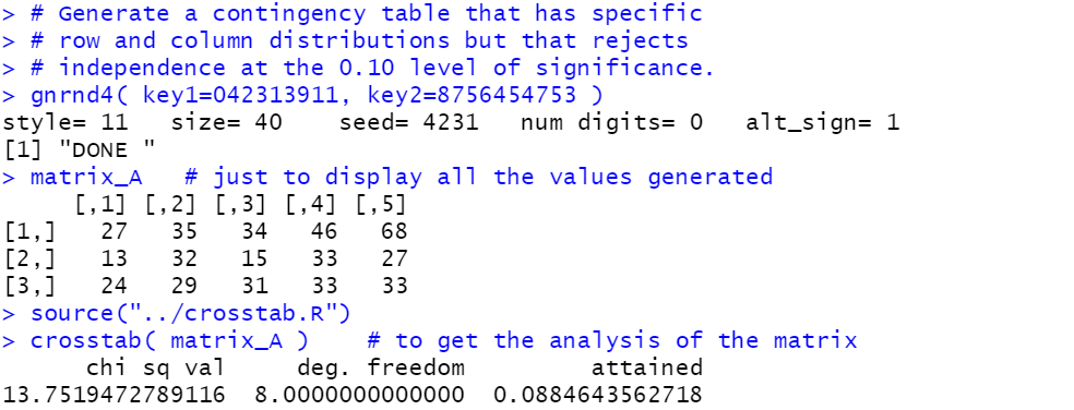
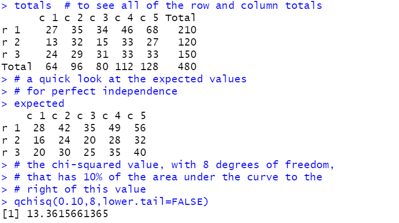
Here is the R console output from the above commands:

Looking at the expected value table we can see that each column has the desired 7:4:5 proportion, and each row has the desired 4:6:5:7:8 proportion. The generated table is slightly off from the expected values. In fact, from the crosstab() function output we can see that the computed chi-squared value is 13.7519472789116 which is just slightly larger than the critical value that we found from the qchisq() function, namely, 13.3615661365, and as a result we would reject independence at the 0.10 level of significance.

Formal description of key values

Key 1	d	d d d d d	d d	d d
	num digits	initial seed value	(generated sample size)-1	style
	Number of decimal digits implied in some second key values and used in generating the actual values in some cases. Also used to determine if certain second key values are negative. Values 0, 1, 2, 3, and 4 represent, respectively 0, 1, 2, 3, or 4 decimal digits. Values 5, 6, 7, 8, 9 represent, respectively, 0, 1, 2, 3, or 4 decimal digits, but with the understanding that some second key values may be negative.	The initial seed value. Generally this is determined by some other random number generator. The value used here then determines the sequence of random values generated by the appropriate functions both in the TI-83/84 program and in the web page.	One less than the desired sample size. Thus a pair of digits such as 11 will generate a 12 item sample, a pair of digits such as 99 will generate a 100 item sample, and a pair of digits such as 00 will generate a 1 item sample.	The style selector. This gives us room for up to 99 different styles of samples. Initially there are 10 defined styles, As more styles are specified this list will expand, Current styles are Uniform Power Root Normal Bi-modal (mixed normal) Linear Regression Discrete Contingency table - first methodology Quartile points Paired Normal Contingency Table - seccond methodology In general, the particular style chosen determines the meaning of the second key.

Style	Name	Text
01:	Uniform	A uniform distribution gives an equally likely probability of having each permissible greater than or equal to some specified Low value and a High value determined to be the Low+Range for some specified Range, This is accomplished by taking a uniformly distributed random value between 0 and 1 and applying it to the Range, adding the result to the Low value, and then rounding the result to the specified number of digits.
02:	Power	This power distribution is identical to the uniform distribution except that the random value that is generated is squared before it is used to scale the Range. The result, since the random values generated initially are between 0 and 1, is to have a distribution that favors low values.
03:	Root	This power distribution is identical to the uniform distribution except that we take the quare root of the random value that is initially generated before it is used to scale the Range. The result, since the random values generated initially are between 0 and 1, is to have a distribution that favors high values.
Key 2	d d d d d d		d d d d d
	These six digits specify the Range of values that may be generated. Note that the number of decimal digits specified in Key 1 places an implied decimal point within the specified digits. Thus, the value 000100 (which could be specified simply as 100) would mean, 100 if the number of decimal digits in Key 1 is 0 or 5. On the other hand, 100 would mean 0.100 if the number of decimal digits in Key 1 is 3 or 7.		These five digits represent the Low end of the permisible values to be generated. Note that if the number of digits specied in Key 1 came from a value greater than 4 then this Low values is set to be a negative, Thus, 20000 with the number of decimal digits given as a 6, has an implied decimal value of 200.00, but it is a negative value, that is, -200.00.

Style	Name	Text
04:	Normal	The program generates values that are approximately normally distributed with a specified mean and a specified standard deviation.
Key 2	d d d d d		d d d d d
	These five digits specify the goal Standard Deviation of values to be generated. Note that the number of decimal digits specified in Key 1 places an implied decimal point within the specified digits. Thus, the value 000100 (which could be specified simply as 100) would mean, 100 if the number of decimal digits in Key 1 is 0 or 5. On the other hand, 100 would mean 0.100 if the number of decimal digits in Key 1 is 3 or 7.		These five digits specify the goal Mean of values to be generated. Note that if the number of digits specied in Key 1 came from a value greater than 4 then this Mean values is set to be a negative, Thus, 20000 with the number of decimal digits given as a 6, has an implied decimal value of 200.00, but it is a negative value, that is, -200.00.

Style	Name	Text
05:	Bi-Modal	The program generateS values that are randomly selected from two approximately normal distributions, each with its own specified mean and standard deviation. Key 2 will give the mean and standard deviation for one distribution, while Key 3 will give the mean and standard deviation for the other distribution. As it generated each value, the process randomly selects which distribution to use. As such, the number of values from each distribution is a random choice and there is no attempt to have an approximately equal number of values from each distribution.
Key 2	d d d d d		d d d d d
	These five digits specify the first goal Standard Deviation of values to be generated. Note that the number of decimal digits specified in Key 1 places an implied decimal point within the specified digits. Thus, the value 000100 (which could be specified simply as 100) would mean, 100 if the number of decimal digits in Key 1 is 0 or 5. On the other hand, 100 would mean 0.100 if the number of decimal digits in Key 1 is 3 or 7.		These five digits specify the first goal Mean of values to be generated. Note that if the number of digits specied in Key 1 came from a value greater than 4 then this Mean values is set to be a negative, Thus, 20000 with the number of decimal digits given as a 6, has an implied decimal value of 200.00, but it is a negative value, that is, -200.00.
Key 3	(-) d d d d d		d d d d d
	These five digits specify the goal Standard Deviation of values to be generated. Note that the number of decimal digits specified in Key 1 places an implied decimal point within the specified digits. Thus, the value 000100 (which could be specified simply as 100) would mean, 100 if the number of decimal digits in Key 1 is 0 or 5. On the other hand, 100 would mean 0.100 if the number of decimal digits in Key 1 is 3 or 7. The negative sign, if present has no effect on the standard deviation, rather, if there is a leading negative sign then the value of the mean, the last five digits, is made negative.		These five digits specify the second goal Mean of values to be generated. Note that, unlike the first goal mean, this one is turned negative by preceding the specified value with a negative sign.

Style	Name	Text
06:	Linear	The linear distribution generates pairs of values, (x,y), such that there is a y=mx+b underlying relationship between the values. To generate our distribution we need to have a Low value for the x-values, a Range for the x-values, a specification for the linear relationship, given as Dy =Mx+B, and an indicator for the maximum amount of error to introduce. The Low and Range values are given in Key 3 while the other valeus are specified in Key 2.
Key 2	d	d	d	d d d	d d	d d
	This is a single digit error factor. To calculate the maximum allowed error on any one observation, if E is this digit, find (E+1)(E+2)/200 and apply that to the max change in the model from the Left x value to the Right x value.	This digit indicates the sign of the B value: 0-5=positive; 6-9=negative.	This digit indicates the sign of the M value: 0-5=positive; 6-9=negative.	These three digits give the value of B in Dy=Mx+B, possibly negated from earlier indicator.	These two digits give the value of M in Dy=Mx+B, possibly negated from earlier indicator.	These two digits give the value of D in Dy=Mx+B.
Key 3	d d d d d			d d d d d
	These 5 digits give the Range of the x-values. Note that this value is scaled by the number of decimal digits specified in Key 1.			These 5 digits give the Low value of the x-values. Note that this value is scaled by the number of decimal digits specified in Key 1. In addition, this value may be changed to a negative value based on that same Key 1 value.

Style	Name	Text
07:	Discrete		The discrete distribution generates values from 1 to the number of categories in an approximation to the relative frequency given for each of the categories. There should be at least two categories and there can be as many as nine categories. The number of categories and the relative frequencies, as single digits, for each category are given in Key 2.
Key 2	d	d	d	d	d	d	d	d	d	d
Key 2	Relative Freq cat 9	Relative Freq cat 8	Relative Freq cat 7	Relative Freq cat 6	Relative Freq cat 5	Relative Freq cat 4	Relative Freq cat 3	Relative Freq cat 2	Relative Freq cat 1	# of cat

Style	Name	Text
08:	Table		The Table distribution fills a table with the number of times a value has been observed in each cell of the table. This is done with a goal of having a certain relative frequency in each row and certain relative frequency in each column of the table. The second Key gives the number of rows and the number of columns, along with a relative frequency of each. The specification below for that second key implies that the sum of the number of rows and number of columns should not excede eight (8). In fact, it can be 9. A further note is that the actual number of "observations" is equal to the "size" as given in Key 1 times the number of rows times the number of columns. This is done because having so many cells in a table means that the "observations" are spread out over many cells. Using this factor approach allows us to get much larger values.
Key 2	d	d	d	d	d	d	d	d	d	d
	Relative Freq col n	Relative Freq col n-1	Relative Freq col n-2	Relative Freq	Relative Freq	Relative Freq	Relative Freq row 2	Relative Freq row 1	# of cols	# of rows
	As implied above, these 8 digits hold the relative frequencies of the rows and columns. Reading right to left we find the relative frequency of row 1, row 2, and so on until we are done with the row values. Then we start with the column relative frequencies. Since there are but 8 digits in this group, we want the number of rows plus the number of columns to be no more than 8. The actual limit is 9, but the documentation here is a bit easier if we show only 8.

Style	Name	Text
09:	Quartile	The Quartile Points distribution chooses random values from the Low value to the Low+Range value such that we have Quartile points set at a specified percent across the range of values. Thus, we could have a range of 300 and specify quartile widths (i.e., the span) at 50%, 15%, 25%, and 10%. These correspond to a span of 150, 45, 75, and 30. The range of values is divided accordingly. Quartile points are set, remaining values are allocated. The values are placed in the list in random order. Also, If the IQR is such that 1.5*IQR does not cover the first or fourth quartile, then the program ensures that there is one point in the outlier region. Finally, the specified size for the sample is always rounded up to one less than the next multiple of 4.
Key 2	pp	pp	pp	d d d	d d d
Key 2	This is the percent of the range given to the first quartile.	This is the percent of the range given to the second quartile.	This is the percent of the range given to the third quartile. Note that the fourth quartile gets the remaining part of the range.	These three digits give the range, possibly altered by the number of decimal digits.	These three digits give the low value, possibly altered by the number of decimal digits.

Style	Name	Text
10:	Paired Normal	The program generates values that are approximately normally distributed with a specified mean and a specified standard deviation. In addition, the program generates a second list with values paired to the first list.
Key 2	d d		d d d d d	d d d d d
Key 2	These two digits specify the spread of the paired values. In particular, values near 00 produce almost no spread while values near 99 produce a great spread and one that is shifted to have the second value tending to be greater than the first.		These five digits specify the goal Standard Deviation of values to be generated. Note that the number of decimal digits specified in Key 1 places an implied decimal point within the specified digits. Thus, the value 000100 (which could be specified simply as 100) would mean, 100 if the number of decimal digits in Key 1 is 0 or 5. On the other hand, 100 would mean 0.100 if the number of decimal digits in Key 1 is 3 or 7.	These five digits specify the goal Mean of values to be generated. Note that if the number of digits specied in Key 1 came from a value greater than 4 then this Mean values is set to be a negative, Thus, 20000 with the number of decimal digits given as a 6, has an implied decimal value of 200.00, but it is a negative value, that is, -200.00.

Style	Name	Text
11:	Independence		The Independence distribution fills a table with the number of times a value has been observed in each cell of the table. This is done with a goal of having a certain relative frequency in each row and certain relative frequency in each column of the table. Furthermore, the table is changed from prefectly independent to failing the test for independence at a given level of significance. The second Key gives the number of rows and the number of columns, along with a relative frequency of each. The specification below for that second key implies that the sum of the number of rows and number of columns should not excede eight (8). In fact, it can be 9. A further note is that the expected number of "observations" is determined by the expected values, which are just the product of the row expected proportion and the column expected proportion. However, a multiplier is used to be sure that the lowest expected value is more than 10. A further aberation is that we determine the goal significance level at which the resuting table will just fail a chi-squared test for independence. That goal level is computed as the first key `generated sample size` divided by 400. Thus the two digit sample size 99 produces a desired sample size of 100 and thus a goal value of 100/400=25%, and the two digit sample size 09 produces a desired sample size of 10 and thus a goal value of 10/400=2.5%.
Key 2	d	d	d	d	d	d	d	d	d	d
	Relative Freq col n	Relative Freq col n-1	Relative Freq col n-2	Relative Freq	Relative Freq	Relative Freq	Relative Freq row 2	Relative Freq row 1	# of cols	# of rows
	As implied above, these 8 digits hold the relative frequencies of the rows and columns. Reading right to left we find the relative frequency of row 1, row 2, and so on until we are done with the row values. Then we start with the column relative frequencies. Since there are but 8 digits in this group, we want the number of rows plus the number of columns to be no more than 8. The actual limit is 9, but the documentation here is a bit easier if we show only 8.