Getting Measures from Grouped Data

Please note that at the end of this page there is a listing of the R commands that were used to generate the output shown in the various figures on this page.

There are times when we are given some summary values and we are asked to calculate some descriptive measures from those values. For example, consider the information in Table 1.

R has no problem dealing with huge collections of values. Therefore, we will take this second approach. Let us examine the new, static, report of grouped values shown in Figure 1.

Figure 1

There are really only 7 midpoint values and 7 frequencies that we need to get into our R session. There is no pattern to the frequencies Therefore we are pretty much stuck with using a statement such as freq<-c(17,35,32,21,12,16,33). We could do the same thing with the midpoint values, namely, mp<-c(30.5,49.5,68.5,87.5,06.5,125.5,144.5). Because they fall into such a nice pattern, there are other ways to generate the same values. One such alternative would be to use the seq() function in the form alt_mp <- seq(from=30.5,to=144.5,by=19). All of these are shown in Figure 2.

Figure 2

What remains to be done is to create the long list of values, 17 instances of 30.5, 35 instances of 49.5, 32 instances of 68.5, and so on. Fortunately, R has a command to do just that. The rep() function, short for replicate, takes care of just such a situation. For our example, we use x<-rep(mp,freq) to replicate each value in mp the number of times given in the corresponding position of freq. The full statement stores the generated data values in the variable x. Figure 3 shows the console view of this statement and of the statement to display the values stored in x.

Figure 3

Now that the long list has been created we can just move ahead to have R compute whatever values we want. For example, Figure 4 shows the commands to find the mean, median, sample standard deviation, and sample variance.

Figure 4

It is important to recall that these computed values represent at best an approximation to the 166 values that were behind the creation of the intervals shown in Table 3. We are using the midpoint of each interval as our best approximation to what the values may have been. Those approximations could be way off.

For example, consider the values generated in Figure 5.

Figure 5

If we install the collate3() function that we saw in an earlier page then we can use that function to build a frequency table from that data. This is shown in Figure 6.

Figure 6

The frequency table displayed in Figure 6 gives much more than the simple counts that we saw back in Figure 1 (Table 3). However, the intervals and the frequencies are identical. The values in new_x could have generated Table 3. However, if we do our simple computations on the values in new_x, as shown in Figure 7, we get values different from those that we found back in Figure 4.

Figure 7

In particular, the mean and median are quite different, although the standard deviation did not change.

Using a different set of data, generated in Figure 8, we can get quite different results.

Figure 8

We can use collate3() to verify that this new data still produces the same frequency chart that we had in Figure 1.

Figure 9

But when we run our simple computation on this new data we get yet other results, as shown in Figure 10.

Figure 10

This time the standard deviation is quite different, the mean is at least close to the original value, and the median is now on the other side of the the original value.

The lesson to learn is that if at all possible work from the original data, not from a summary of it. Before we had computers, performing computations on huge collections of data was daunting to say the least. Now, with computers, there is no reason not to use the original data.

Here is the list of the commands used to generate the R output on this page:

# the commands used on frimgrouped.htm
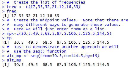
#  Create the list of frequencies
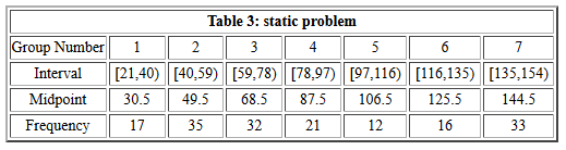
freq <- c(17,35,32,21,12,16,33)
freq
#  Create the midpoint values.  Note that there are 
#  many different ways to generate these values.
#  Here we will just enter them as a list.
mp<-c(30.5,49.5,68.5,87.5,106.5,125.5,144.5)
mp
#  Just to demonstrate another approach we will
#  use the seq() function
alt_mp <- seq(from=30.5,to=144.5,by=19)
alt_mp
#
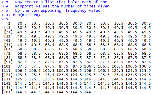
#   Now create a list that holds each of the
#   midpoint values the number of times given
#   by the corresponding  frequency value
x<-rep(mp,freq)
x
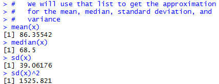
#   We will use that list to get the approximation
#   for the mean, median, standard deviation, and 
#   variance
mean(x)
median(x)
sd(x)
sd(x)^2
#
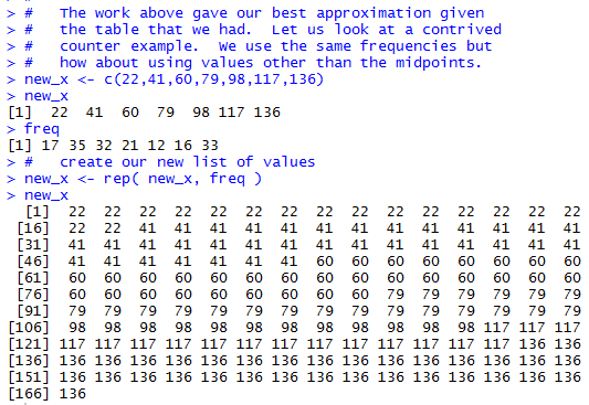
#   The work above gave our best approximation given
#   the table that we had.  Let us look at a contrived
#   counter example.  We use the same frequencies but 
#   how about using values other than the midpoints.
new_x <- c(22,41,60,79,98,117,136)
new_x
freq
#   create our new list of values
new_x <- rep( new_x, freq )
new_x
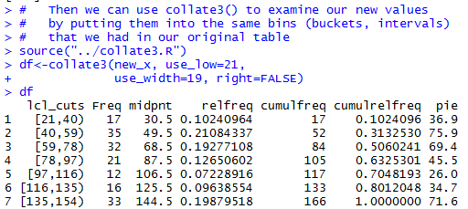
#   Then we can use collate3() to examine our new values
#   by putting them into the same bins (buckets, intervals)
#   that we had in our original table
source("../collate3.R")
df<-collate3(new_x, use_low=21,
             use_width=19, right=FALSE)
df
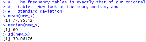
#   The frequency tables is exactly that of our original
#   table.  Now look at the mean, median, abd
#   standard deviation
mean(new_x)
median(new_x)
sd(new_x)
#
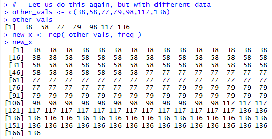
#   Let us do this again, but with different data
other_vals <- c(38,58,77,79,98,117,136)
other_vals
new_x <- rep( other_vals, freq )
new_x
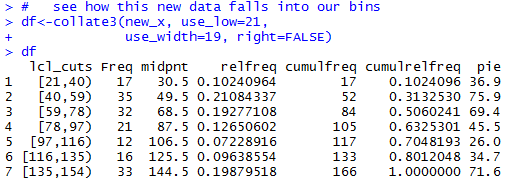
#   see how this new data falls into our bins
df<-collate3(new_x, use_low=21,
             use_width=19, right=FALSE)
df
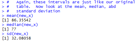
#   Again, these intervals are just like our original
#   table.  Now look at the mean, median, abd
#   standard deviation
mean(new_x)
median(new_x)
sd(new_x)
#