Typical Problem Steps (on a PC)
Return to Topics page
This page, written first in August 2016, is meant to serve as a model for how
we will be doing most of our work in this class.
Note that some of the screen images have been altered to highlight
certain features.
In general, we will
- be given some data in a table
- need to generate that data in a RStudio session
- be give some questions about the data or requests to produce
some graphs of the data
- need to find a way to have R produce answers to
those questions or to produce the
requested graphs.
In the Fall 2016 term, students will have been given a
USB drive that starts out with copies of my special files for
students to use in the course.
Furthermore, we will do all of our work on
those USB drives. It will be most convenient if,
for each problem that we want to do we
create a separate folder on the UBS drive to hold all of our work for that
problem.
This page will step through doing this on a PC.
We are asked to find the mean, median and mode of the data.
We plug in our USB drive.
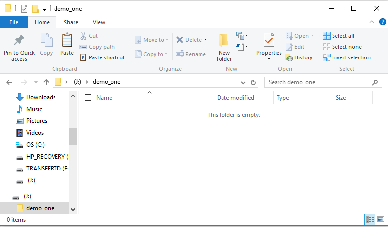
On a PC this should open a File Explorer
window such as the one shown in Figure 1.
Figure 1
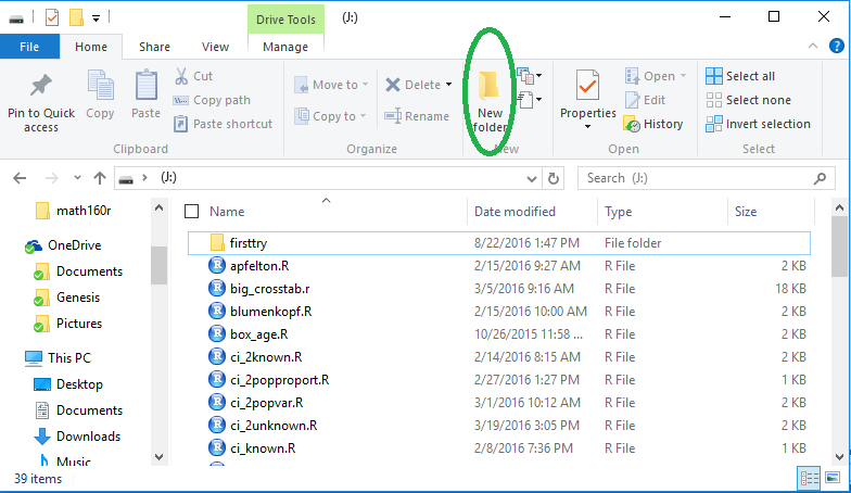
The files on the USB drive hold various function that have been given to you.
The existing folder, firsttry, was created when we installed and tested
RStudio.
Now, to do this demonstration, we want a new folder.
To create the new folder we click on the
 icon that has been highlighted in
Figure 1.
This creates the new folder shown in Figure 2.
icon that has been highlighted in
Figure 1.
This creates the new folder shown in Figure 2.
Figure 2
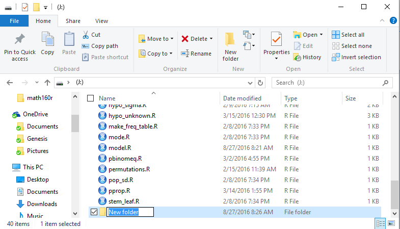
The proposed title of the new folder, namely, New folder,
should be replaced by something more meaningful. We will use
demo_one which we just type into the folder
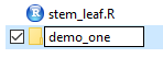
name space as shown in Figure 3.
Figure 3
Our next step is to create a file in that new folder. The file
should have an .R extension. Also, we want the file to
contain a valid R statement.
Rather that go through a lot of work to do this, we have a model of
such a file on the USB drive. We can just copy that file to our new
directory.
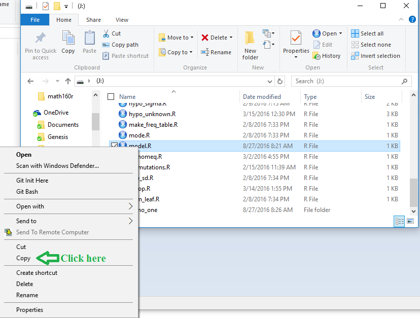
Figure 4 shows where we right click on the name of the file,
model.R,
to get the options shown in the window on the lower left.
Click on the Copy option.
Figure 4
Now that we have a copy of model.R
we want to place that copy into the
demo_one folder.
Therefore, still in Figure 4, we locate the demo_one
folder icon,  , and double click on
it to open the screen shown in Figure 5.
, and double click on
it to open the screen shown in Figure 5.
Figure 5
We just created this folder so there is nothing in it.
Point to the empty part of the screen and right click
there to open the window shown in
Figure 6.
Figure 6
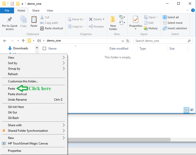
In the window shown in Figure 6 click on the
Paste option.
That places the copy of the file into the folder.
Figure 7
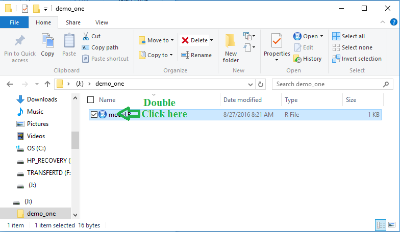
Now, with this file, model.R, in our directory
we can double click on it to open a new RStudio session
shown in Figure 8.
Figure 8
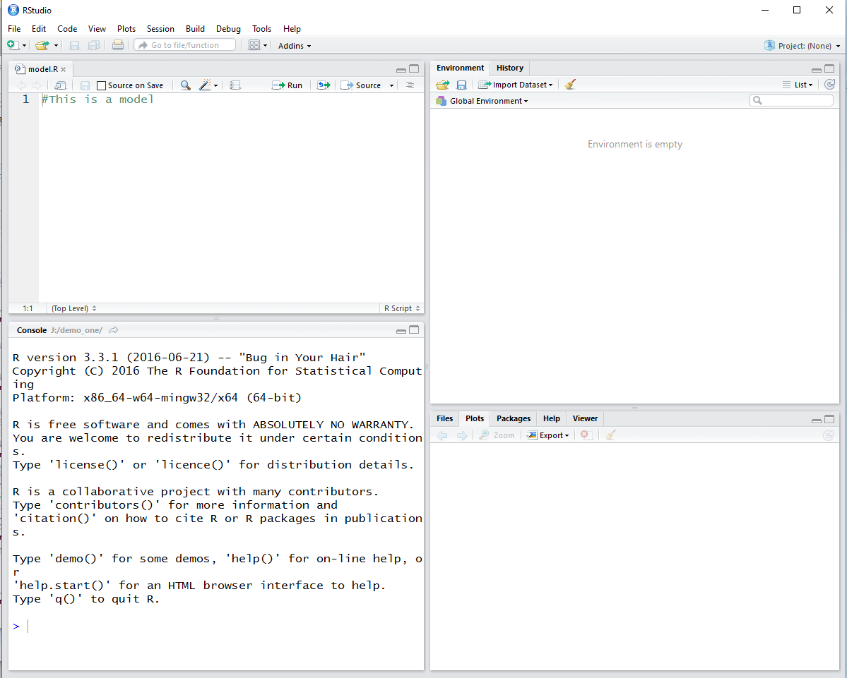
As we see in Figure 8, the editor window is open and it shows
the contents of our model.R file.
There are no variables defined in the environment pane.
Only the splash screen is in the Console pane.
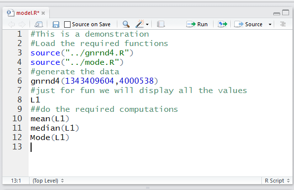
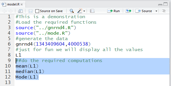
We will change the model.R edit screen to hold the following
lines
#This is a demonstration
#Load the required functions
source("../gnrnd4.R")
source("../mode.R")
#generate the data
gnrnd4(1343409604,4000538)
#just for fun we will display all the values
L1
##do the required computations
mean(L1)
median(L1)
Mode(L1)
Things to note:
- The use of upper and lower case letters is important.
- Once R finds a # character R considers that
character and anything after it on that line to be a comment.
We should use comments to explain what we are doing.
- You can just type the lines into the editor pane or
you could copy the lines from this page and just paste them into the editor pane.
- The editor is just that. Nothing happens just because the lines ae in the editor pane.
- The editor colors different components in different ways. This
helps us to identify some mistakes should we make them.
- Just becasue the lines are in the editor pane it does not mean that the
lines have been saved to the file. That takes a separate action.
Figure 9
In Figure 9 we see that the new lines have been placed into the editor
pane. Now would be a good time to save this work to the model.R
file. To do this we need only click on the  icon.
icon.
Once the lines have been saved we can look at the Files tab
in the lower right pane of the RStudio window.
In Figure 10 we see that the model.R
is there, that it has been updated with a new date and time stamp, and that its size
is shown as more than just a few characters.
Figure 10
Back in the editor pane, we can highlight our first command,
source("../gnrnd4.R") so that we can perform it.
This command will look at the directory (folder) above our current directory
to find a file called gnrnd4.R and the command will run
the commands that are in that file.
The gnrnd4.R file contains R
commands that I wrote to accomplish certain tasks.
We will make repeated use of those commands.
Once the source("../gnrnd4.R") command is highlighted we
click on the  icon to actually run the command.
Figure 11
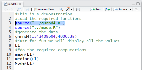
Figure 12 shows the result in the Console pane.
We see that the command has appeared here and that it has been performed.
[The fact that there is no error message means that it
performed without an error.]
Figure 12
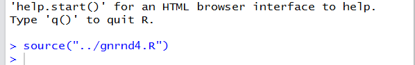
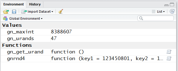
Figure 13 shows the Environment pane. Here we see that running the
commands in the gnrnd4.R file caused two ne variables to be created and
given some strange values, and it caused two new functions to be created, one
is called gn_get_urand and the other is called
gnrnd4.
Figure 13
While we are at it, we might as well perform the second
command, source("../mode.R"). Again, in the editor pane we highlight the command,
as shown in Figure 14 and then we press the
icon.
Figure 14
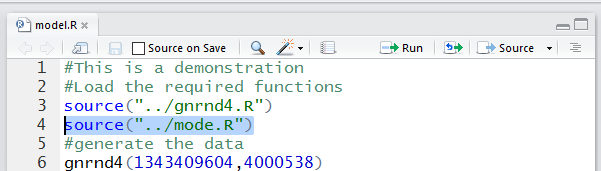
Figure 15 shows the updated Console pane.
Figure 15
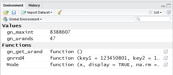
Figure 16 shws the updated Environment pane.
There we see that a new function, Mode, has been defined.
Figure 16
We return to the Editor pane and highlight the next command,
gnrnd4(1343409604,4000538). That command came from the original problem
statement at the start of this page. There we were given a table of data.
At the bottom of the table we were told that we could generate the same
data by using the gnrnd4 function along with two key values,
1343409604 and 4000538. To do that we create the command
gnrnd4(1343409604,4000538) and then we use the
icon to run it.
Figure 17
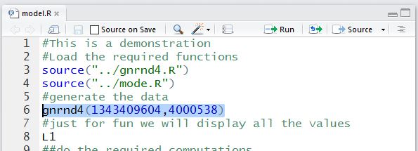
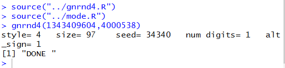
Figure 18 shows the update of the Console pane.
Performing this command produced some output and a
final "Done" indication.
Figure 18
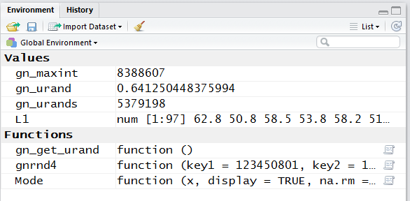
The real result of running the command is relected
in the update of the Environment ane.
This is shown in Figure 19.
First note that there are some new variables.
Second note that the value of the variable gn_urands
has changed from what it was back in Figure 16.
Third, note that we new variable L1
holds numeric values and it holds 97 such values.
Also, the first five of those values are identical to the values that
we in our original table of values.
Figure 19
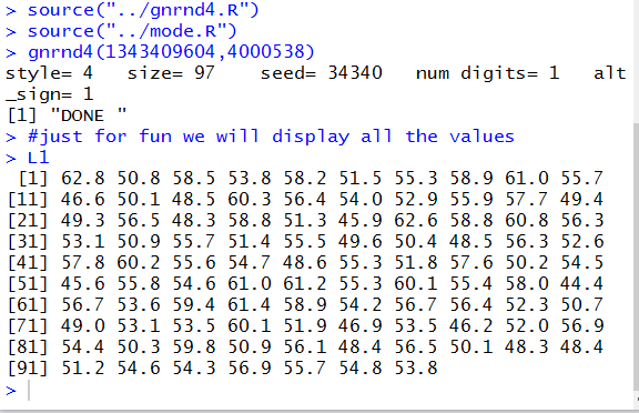
We can get R to display all of the values by using the command
L1. In the Editor pane we have highlighted the comment and that command.
Then we click on the
icon to run those two lines.
Figure 20
In Figure 21 we see that the comment
has appeared as is. That is followed by all 97
values in the variable L1.
Each line of the listing of values starts with a number in square brackets.
That number tells us the position
within the variable L1
of the first value displayed in that output line.
Thus, 62.8 is in position 1, 46.6 is in position 11, 49.3 is in position 21, and so on.
Figure 21
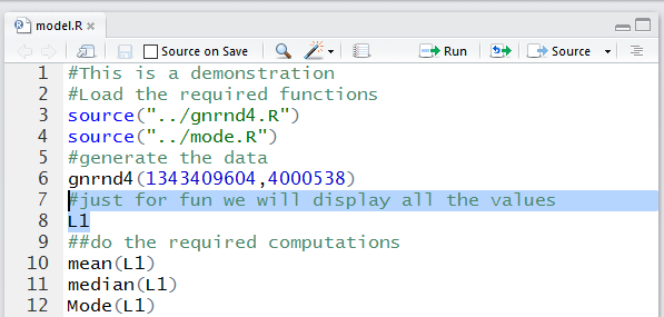
We can return to the Editor pane
and highlight the remaining lines.
[Just as a note, mean and median are functions that
are part of the R language. Mode, on the other hand,
is not a part of the language. I had to write special commands to get R
to be able to find the mode of a set of data. We have loaded Mode
into our workspace so we can now use it.]
Figure 22
Then click on icon to run those lines.
Figure 23
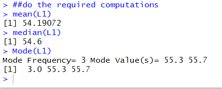
The output from the mean(L1) and median(L1)
commands is clear. The mean value is 54.19072 and the median value is 54.6.
The output from the Mode(L1) command tells us that there
were two values, 55.3 and 55.7, that each appeared 3 times and that
no other value appeared that oftern or more often.
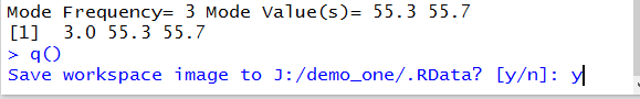
We have finished our assignment. We are ready to close RStudio.
We use the q()command and R
responds by asking if we should save the workspace.
We say y and press the Enter key to
end the session.
Figure 24
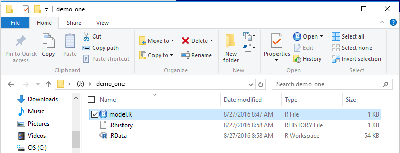
Back in the File Explorer window, shown in Figure 25, we now see that
we have the two "hidden" files added to the folder.
this means that if we start RStudio from this folder,
by double clicking the model.R file, our workspace, inclucing the variables
and the functions that we have loaded, will be right back where
they were when we finished in Figure 24.
Figure 25
Return to Topics page
©Roger M. Palay
Saline, MI 48176 August, 2017