Confidence Interval for the Population Standard Deviation

Return to Topics page
On this page we look at creating a confidence interval for the population standard deviation or variance based on a sample standard deviation. We will do this for cases where we have a strong belief that the underlying population is approximately normal.

For populations that are approximately normal and for samples of size n the ratio of the quantity (n-1)s² to σ² is distributed as a χ² with n-1 degrees of freedom. The consequence of this is that for a sample of size n with a sample standard deviation of s_x we can find a 95% confidence interval for the population standard deviation, σ, by computing the two values

and

, both for a χ² with n-1 degrees of freedom and where we understand that

represents the x-value that has an area equal to 0.025 to its right and

represents the x-value that has an area equal to 0.025 to its left. You might note a seeming inversion here. The lower value for the confidence interval,, uses the area on the right, while the upper value of the confidence interval, , uses the area on the left. This inversion is the result of having the χ² critical values in the denominator. We know that the χ² value on the left will be a smaller value than the one on the right. Therefore, when we divide the numerator by those values the division by the larger denominator produces a smaller quotient.

We can walk through an example here. Let us say that for an apparently normal population we have a sample of size 34 and the sample standard deviation is 4.71. We want to generate a 95% confidence interval for the population standard deviation. The χ² distribution that we will use is the one with 34-1 or 33 degrees of freedom. The following commands in R will compute and display the values that we need.

lval <- qchisq(0.025,33)
lval
rval <- qchisq(0.025, 33, lower.tail=FALSE)
rval
s<-4.71
s
sqrt(33*s*s/rval)
sqrt(33*s*s/lval)

The console view of those commands is shown in Figure 1.

Figure 1

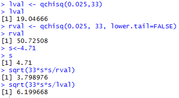
Thus, the 95% confidence interval generated by our sample, is (3.799,6.200), rounded to three decimal places.

This model can be used to do any other problem. For example, to find the 90% confidence interval for the population standard deviation from a sample of size 16 where the sample standard deviation is 1.388, we would use the commands

lval <- qchisq(0.05,15)
lval
rval <- qchisq(0.05, 15, lower.tail=FALSE)
rval
s<-1.388
s
sqrt(15*s*s/rval)
sqrt(15*s*s/lval)

The console view of those commands is shown in Figure 2.

Figure 2

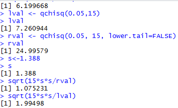
Thus, the 90% confidence interval generated by our sample, is (1.075,1.995), rounded to three decimal places.

Considering that we are doing the same steps every time we find a problem asking for the confidence interval for the population mean based on a sample standard deviation, this looks like a perfect time to create a function to do these steps for us. Here is the text of such a function.

ci_stddev <- function(  n=30, s=0, cl=0.95)
{
  # try to avoid some common errors
  if( cl <=0 | cl>=1)
  {return("Confidence interval must be strictly between 0.0 and 1")
  }
  if( s <= 0 )
  {return("Sample standard deviation must be positive")}
  if( n <= 1 )
  {return("Sample size needs to be more than 1")}
  if( as.integer(n) != n )
  {return("Sample size must be a whole number")}
  # to get here we have some "reasonable" values
  alpha = (1-cl)/2 # area at each side
  lval <- qchisq(alpha,n-1)
  rval <- qchisq(alpha,n-1,lower.tail=FALSE)
  low_end <- sqrt((n-1)*s*s/rval)
  high_end <- sqrt((n-1)*s*s/lval)
  result <- c(low_end, high_end, n-1, lval, rval)
  names(result)<-c("CI Low","CI High","deg. of freedom","left chisq", "right chisq")
  return( result )
}

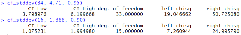
The function is also available in the file ci_stddev.R. Figure 3 shows two instances of the new function, one for each of the problems that we solved above. Fortunately, we get the same results as before.

Figure 3

There is one more aspect of this confidence interval that is worth noting. Unlike the confidence intervals that we had for the population mean, these confidence intervals are not symmetric about the point estimate that we have. Thus, in the last example, the confidence interval was (1.075,1.995) and our point estimate was the sample standard deviation, 1.388. But 1.388 is not the midpoint of the confidence interval. We have a width to the interval, 1.995-1.075 = 0.92 in this case, but we do not have that same sense of a margin of error.

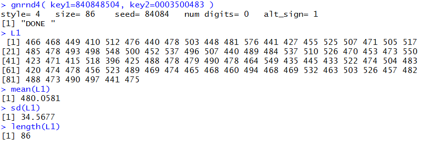
One last, complete example may help. Consider the values in Table 1 which represent a sample of values from a population that we happen to know to be approximately normally distributed. However, we do not know the population mean, μ, or its standard deviation, σ.
We can create this same data in R and find both the mean and the sample standard deviation, along with the size of the sample. This is done in Figure 4.

Figure 4

Now that we know those three values we could construct a 90% confidence interval for the population mean. We can do this in a step by step approach or we can use the function that we created in an earlier page, ci_unknown(). Assuming that we have "loaded" that function it seems to be the better approach. Figure 5 shows the use of that function and the resulting values.

Figure 5

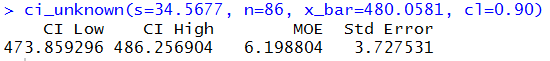
Our interpretation of the result is to say that we have a confidence interval of (473.60,486.26) and that 90% of the confidence intervals that we produce this way contain the true population mean. We note that the sample mean, 480.06 is in the middle of the confidence interval and that the margin of error is 6.20 (all values rounded to 2 decimal places).

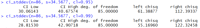
We can use the same data to generate a 90% confidence interval for the population standard deviation. Again, we could go through the step by step process shown above, or we could use the function ci_stddev() that we just developed. Assuming that we have "loaded" that function it seems to be the better approach. Figure 6 shows the use of that function and the resulting values.

Figure 6

Our interpretation of the result is to say that we have a confidence interval of (30.735,39.6-6) and that 90% of the confidence intervals that we produce this way contain the true population standard deviation. Naturally, the sample standard deviation, 34.5677 is in the confidence interval although it is not in the middle of the interval.

Just as we have seen in other confidence intervals, if we increase the confidence level, we get wider confidence interval. For example, Figure 7 shows the same computation but with the goal of producing a 95% and then a 99% confidence interval.

Figure 7

R commands used in preparing this web page.

source("../gnrnd4.R")
source("../ci_unknown.R")

lval <- qchisq(0.025,33)
lval
rval <- qchisq(0.025, 33, lower.tail=FALSE)
rval
s<-4.71
s
sqrt(33*s*s/rval)
sqrt(33*s*s/lval)

lval <- qchisq(0.05,15)
lval
rval <- qchisq(0.05, 15, lower.tail=FALSE)
rval
s<-1.388
s
sqrt(15*s*s/rval)
sqrt(15*s*s/lval)

ci_stddev <- function(  n=30, s=0, cl=0.95)
{
  # try to avoid some common errors
  if( cl <=0 | cl>=1)
  {return("Confidence interval must be strictly between 0.0 and 1")
  }
  if( s <= 0 )
  {return("Sample standard deviation must be positive")}
  if( n <= 1 )
  {return("Sample size needs to be more than 1")}
  if( as.integer(n) != n )
  {return("Sample size must be a whole number")}
  # to get here we have some "reasonable" values
  alpha = (1-cl)/2 # area at each side
  lval <- qchisq(alpha,n-1)
  rval <- qchisq(alpha,n-1,lower.tail=FALSE)
  low_end <- sqrt((n-1)*s*s/rval)
  high_end <- sqrt((n-1)*s*s/lval)
  result <- c(low_end, high_end, n-1, lval, rval)
  names(result)<-c("CI Low","CI High","deg. of freedom","left chisq", "right chisq")
  return( result )
}

ci_stddev(34, 4.71, 0.95)
ci_stddev(16, 1.388, 0.90)

gnrnd4( key1=840848504, key2=0003500483 )
L1
mean(L1)
sd(L1)
length(L1)
ci_unknown(s=34.5677, n=86, x_bar=480.0581, cl=0.90)
ci_stddev(n=86, s=34.5677, cl=0.90)
ci_stddev(n=86, s=34.5677, cl=0.95)
ci_stddev(n=86, s=34.5677, cl=0.99)