Confidence Interval for a Population Proportion

Return to Topics page
In the case where we have a population where some of the elements in that population have a specific characteristic, we talk about the proportion of the population that has that characteristic. We generally signify that proportion as p. If we take a sample of size n of that population and in that sample we find x items with the characteristic, then the value

is a point estimate for p. We want a confidence interval for p derived from the sample. That confidence interval will be point estimate ± (margin of error)
± (margin of error) The we recall that for cases where n*p≥10 and n*(1-p)≥10 we have the distribution of

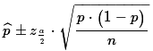
is normal with mean = p and standard deviation = √p*(1-p)/n. Therefore, for a specified confidence level we can find z_α/2 to make the margin of error = 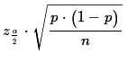That makes the confidence interval be

Of course, the problem with this is that we do not know the value of p so we cannot compute that formula.

Instead, if we change our special conditions, we can use

instead of p in the approximation of the standard deviation. The new restrictions are

The sample size n is no more than 5% of the population size. (Another, popular, way to say this is that the population size is more than 20 times the sample size, n.)
Population items either have the characteristic or the do not. That is another way of saying that the population items fall into one of two categories, those with the characteristic and those without the characteristic.
The sample must contain at least 10 items in each of the two categories.

If these conditions are met then we can use

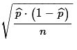as the approximation of the standard deviation of the

's. That gives the formula

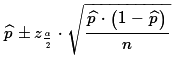to use to find the desired confidence interval for the population proportion p based on a sample of size n with x items in the sample having the characteristic so that =x/n.

An example is in order here. We start with a population of enormous size, something having over 20,000 items. We take a sample of size 73 (this is less than 5% of the population so we are OK on that point). Of the 73 items, 17 have a certain characteristic. That means that 73-17=56 items do not have the characteristic. (There are more than 10 items that do and 10 items that do not have the characteristic in the sample. , so we are OK on that point). Then we can compute an approximation to the sample proportion as 17/73 ≈0.233, which means that (1-) ≈ 0.767. We use those values to compute an approximation to the standard deviation of sample proportions as √p*(1-p)/n = √0.233*0.767/73 ≈ 0.049.

To find the 95% confidence interval from 17 items out of 73 in the sample, we need to find the z_α/2 that gives us 95% of the area under the curve between z_α/2 and -z_α/2. We can use the table, a calculator, or the qnorm(.025) statement to do this. That value turns out to be 1.96. With all that the confidence interval becomes 0.233 ± 1.96*0.0.049 ≈ 0.233 ±0.096 or (0.137,0.329). All that computation is captured in the R statements:

x <- 17
n <- 73
p_hat <- x/n
p_hat
p_hat_sd <- sqrt(p_hat*(1-p_hat)/n)
p_hat_sd
alpha_div_2 <- (1-0.95)/2
alpha_div_2
z <- abs( qnorm( alpha_div_2))
z
lower <- p_hat - z*p_hat_sd
upper <- p_hat + z*p_hat_sd
lower
upper

Figure 1 shows the console view of performing those statements.

Figure 1

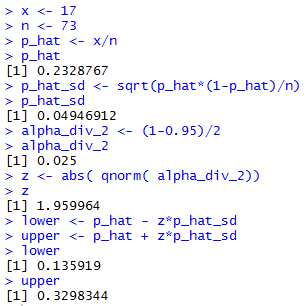
The difference between our earlier hand computed confidence interval and the one shown in Figure 1 is that the former involved some significant rounding in the approximations that we made. The latter still has approximations, but the values are carried for many more digits.

We could do many more examples, but they all follow the same computations shown in Figure 1. As we have done before, we can codify those computations in a function. All we need to do is to feed the function the values of n, p, and the desired confidence interval. Then we let the function perform all of the required computations. One such function is defined by:

ci_prop <- function( n, x, cl=0.95)
{
  # compute a confidence interval for the 
  # proportion given the sample size, the 
  # number of items with the characteristic,
  # and the confidence level
  
  # do a few checks on the information given
  if( cl <=0.0 | cl >= 1 )
  {return("Confidence level needs to be between 0 and 1")}
  if( x < 10)
  {return("Need at least 10 items with the characteristic")}
  if( n-x < 10)
  {return("Need at lease 10 items without the characteristic")}
  # we have no way to check if we are sampling < 5% 
  # of the population
  p_hat <- x/n
  p_hat_sd <- sqrt(p_hat*(1-p_hat)/n)
  alpha_div_2 <- (1-cl)/2
  z <- abs( qnorm( alpha_div_2))
  lower <- p_hat - z*p_hat_sd
  upper <- p_hat + z*p_hat_sd
  if(lower < 0) { lower<-0}
  if(upper > 1 ) { upper <- 1}
  
  result<-c(lower, upper, p_hat, z, p_hat_sd)
  names(result) <- c("lower", "upper", "p hat",
                     "z-score", "p hat sd")
  return( result )
  
}

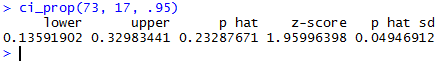
Once defined we can use the statement ci_prop(73, 17, .95) to do all of the work that we saw back in Figure 1. This is shown in Figure 2.

Figure 2

Now that we have the ci_prop() function available it is easy to try out some other situations. Look at what we can learn from doing:

ci_prop(73,10,.95)
ci_prop(73,7,0.95)
ci_prop(73,64,0.95)
ci_prop(73,17,0.90)
ci_prop(73,17,0.80)
ci_prop(73,17,0.99)

The console report on these is given in Figure 3.

Figure 3

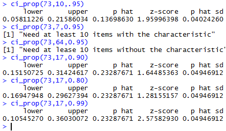
The results shown in Figure 3 illustrate the effect of having a smaller

, of having too small a value for x, of having a too large value for x, and of changing the desired confidence level. Of particular note is the fact that by lowering the desired confidence level we make the confidence interval smaller.

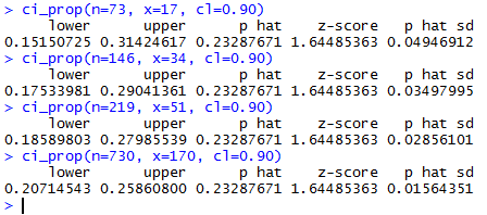
Let us look at making the confidence interval narrower by increasing the sample size. In our original example we found 17 of 73 items have the identified characteristic. If we had a sample of 146 and found 34 with the desired characteristic, then our

would not have changed. However, with the larger sample size we will get a narrower confidence interval. Figure 4 show a few examples where the sample proportion does not change but the sample size does.

Figure 4

We can make the margin of error, half the width of the confidence interval, as small as we want by increasing the sample size. To some extent this is true. Remember that we start with the margin of error = and then realized that we had to use the approximation involving

, namely,

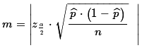We could solve that equation for n to get

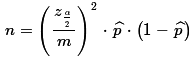This seems to give us a way to determine the required sample size, n, if we have the other values, including a desired margin of error.

The problem with this is that we cannot be sure that we will get the same proportion of items with the specified characteristic in a new sample. If we use the situations illustrated in Figure 4 we see that the proportion is about 0.23287671, really 17/73. If we want a margin of error = 0.02, then the formula we just found tells us that n = (1.64485363/0.02)²*(17/73)(56/73) or about 1208.33. Even if we round that off to 1241, the first whole number larger than 1208 that is evenly divisible by 73, there is no reason why, if we took a sample of 1241 items that we would have the same 17/73 of them, 289 of them, having the specified characteristic. Most likely we will be close, but we just cannot be sure.

One final note here is that although we stated above that the population was enormous, we also qualified that by saying that it had over 20,000 items. If we wanted to take a sample of size 1241 we need to be sure that we are not sampling more than 5% of the population. But 5% of 20,000 is 1,000. We need to be sure that the population has more than 20 times the 1241, that is, 24,820 items in it.
Return to Topics page
©Roger M. Palay Saline, MI 48176 January, 2016