Two Populations; Independent Samples -- Variance
Return to Topics page
Preliminaries
This topic is quite different from the others presented in this section.
-
First, we will be looking at the variance as a parameter
of a population or as a statistic of a sample.
Up to this point we have generally been dealing with the
standard deviation rather than the variance.
Remember that the variance is just the square of the standard deviation.
For populations σ is the standard deviation
and σ2 is the variance.
For samples s is the standard deviation
and s2 is the variance.
-
Second, we will be looking at two populations, and therefore at two
independent random samples,
but the underlying populations must
be normal (or at least approximately normal).
-
Third, in earlier situations when we wanted to look at
a null hypothesis that says two values are identical, i.e., the same,
we looked at the difference of those two as being zero,
as in μ1 - μ2 = 0.
Now, instead of looking at the difference being zero
we will look at the ratio of those values as being one.
Thus, we will be looking at the ratio of values, as in
 or
or
 .
.
-
Fourth, we will be using a new distribution, the F-distribution,
which, if we were using tables of values, would be dramatically more complex
than any distribution that we have seen to this point. However,
since we are using R there is just a slight up-tick in the complexity
of using this new distribution.
The F-distribution
This section is meant to be enlightening, but not a thorough treatment of
the F-distribution. In earlier distributions, the binomial, the normal,
the Student's t, and the χ² we have actually
gone back to looking at values in tables. You may have
noticed the following progression to which we now add the
F distribution.
- normal distribution: We have one standard table
which we can read forward or backward.
The normal distribution is symmetric.
z-values for the normal distribution can be positive or negative,
with the vast majority of the standard normal distribution
lying between the z-values -3 to 3.
In R, rather than read a table, we use the functions pnorm and
qnorm.
The function pnorm(z) gives us the area
under the curve to the left of the z-score z,
i.e., the probability of getting a value less than z in the
standard normal distribution.
The function pnorm(z,lower.tail=FALSE) gives us the area
under the curve to the right of the z-score z,
i.e., the probability of getting a value greater than z in the
standard normal distribution.
The function qnorm(p) gives us the z-score in a standard normal distribution that has
the area under the curve to the left of z being
equal to p, i.e., that has a probability of p
of being less than z.
The function qnorm(p,lower.tail=FALSE) gives us the z-score in a standard normal distribution that has
the area under the curve to the right of z being
equal to p, i.e., that has a probability of p
of being greater than z.
- Student's t distribution: We could have a different standard
distribution table for each different number of degrees of freedom
and we could read these tables forward and backward.
This could easily take 200 pages to print all of the tables in a book
but here we have seen that we could look at any one table for a specific
number of degrees of freedom by going to
Index of Student's t tables
which serves as a gateway to tables for the first 100 degrees of freedom.
However, the practice for textbooks is to have
a single table that just holds critical values for just a few
common percentages.
An example
of such a table can be found at
Critical Values of Student's t.
t-scores for the Student's t distribution can be positive or negative
and the spread of the scores changes with the change in the degrees of freedom.
For lower degrees of freedom the Student's t is
significantly flatter than was the normal distribution. However for large
degrees of freedom the Student's t approaches the normal distribution.
The Student's t distribution is symmetric.
In R, rather than read a table, we use the functions pt and
qt.
The function pt(t,df) gives us the area
under the curve, for df degrees of freedom,
to the left of the t-score t,
i.e., the probability of getting a value less than t in the
student's-t distribution for df degrees of freedom.
The function pt(t,df,lower.tail=FALSE) gives us the area
under the curve, for df degrees of freedom,
to the right of the t-score t,
i.e., the probability of getting a value greater than t in the
student's-t distribution for df degrees of freedom.
The function qt(p,df) gives us the t-score in a
student's-t distribution with df degrees of freedom that has
the area under the curve to the left of t being
equal to p, i.e., that has a probability of p
of being less than t for df degrees of freedom.
The function qt(p,df,lower.tail=FALSE) gives us the t-score in a
student's-t distribution with df degrees of freedom that has
the area under the curve to the right of t being
equal to p, i.e., that has a probability of p
of being greater than t for df degrees of freedom.
- χ² distribution: We could have a different standard
distribution table for each different number of degrees of freedom
and we could read these tables forward and backward.
In a printed textbook this would take many hundreds of pages.
Here we could set things up so that we have a cumulative probability table for
each different number of degrees of freedom. Here is a
link to a page
that asks you for the number of degrees of freedom and then allows you
to generate such a cumulative probability table.
However, the practice is to have
a single table that just holds critical values for just a few
common percentages. A link to a web page of such values is at
The Chi-Squared Critical Values Table.
The χ² distribution is not symmetric.
The x-values of the χ² distribution must be non-negative.
The distribution changes shape with different degrees of freedom.
In an earlier page we saw examples of graphs of various χ²
distributions.
In R, rather than read a table, we use the functions pchisq and
qchisq.
The function pchisq(x,df) gives us the area
under the curve, for df degrees of freedom,
to the left of the χ²-score x,
i.e., the probability of getting a value less than x in the
χ² distribution for df degrees of freedom.
The function pchisq(x,df,lower.tail=FALSE) gives us the area
under the curve, for df degrees of freedom,
to the right of the χ²-score x,
i.e., the probability of getting a value greater than x in the
χ² distribution for df degrees of freedom.
The function qchisq(p,df) gives us the x-score in a
χ² distribution with df degrees of freedom that has
the area under the curve to the left of x being
equal to p, i.e., that has a probability of p
of being less than x for df degrees of freedom.
The function qchisq(p,df,lower.tail=FALSE) gives us the x-score in a
χ² distribution with df degrees of freedom that has
the area under the curve to the right of x being
equal to p, i.e., that has a probability of p
of being greater than x for df degrees of freedom.
- The F distribution: This is a non-symmetric distribution.
We want to look at the ratio of variances in two populations, i.e.,
. In the case where the
two variances, σ1² and
σ2², are equal, that ratio is 1.
If we take samples from the two populations of size n1
and n2, respectively, then we know the resulting ratio of the
sample variances will be close to 1.
(We do not expect it to be 1 because these are only samples.)
The F distribution describes the distribution of values for the ratio of sample
variances in such a case.
The size of each sample has an affect on how well each sample variance
approximates the underlying population variance. As such, the F distribution
has two specifications for the degrees of freedom.
The first degree of freedom is one less than the size of the sample from the numerator
sample and the second degree of freedom is one less than the size of the sample from the
denominator sample.
The ratios, which we will call the x-values for the F distribution,
must be non-negative.
The shape of F distribution changes for different pairs of
degrees of freedom.
This next section presents, in absurd detail, various tables for using the
F distribution. Once we have R we have no need for such tables.
However, part of the course is to see the tables, to learn how to use the tables,
and, to get an even deeper feel for the F distribution by exmining
those tables. In short, if you are in a hurry, just skip over this part,
there is a note similar to this at the end of this part, and just start
looking at the R functions pf() and qf().
|
Tables in general
Recall that we could generate a single table for the standard normal distribution.
Printing such a table would take up at most two pages in a textbook so this is often done.
Then recall that we could generate a table for each different number of degrees of freedom
for a Student's-t distribution. Each such table would take about two printed pages. To do a table
for degrees of freedom from 1 to 100 would take 200 pages so this is never done.
Instead, textbooks show a table of critical values for the
Student's-t distribution. That is, the authors pick out a small number of
supposedly useful probabilities and then present a table that shows the t-values
that have that area to its right. This allows the authors to generate one table
where each line of the table presents the critical values for the Student's-t distribution
for one specific number of degrees of freedom. Such a table takes up no more than 2 pages so this is
quite common in statistics textbooks.
Then recall that we could generate a table for each different number of degrees of freedom
for a χ² distribution. Non each such table might take about eight to ten printed pages. To do a table
for degrees of freedom from 1 to 100 would take 800 to 900 pages so this is never done.
Instead, textbooks show a table of critical values for the
χ² distribution. That is, the authors pick out a small number of
supposedly useful probabilities and then present a table that shows the χ²-values
that have that area to its right. This allows the authors to generate one table
where each line of the table presents the critical values for the χ² distribution
for one specific number of degrees of freedom. Such a table takes up no more than 4 pages so this is
quite common in statistics textbooks.
Returning to our F distribution, we could generate a table for
each different pair of degrees of freedom and we could
read these tables forwards and backwards. This is even worse than you might
imagine in that the area to the left of a specific value,
say 0.44, for the pair of degrees of freedom 15,27 is different from
the area to the left of that same value for
the pair 27,15.
The following image shows part of the table for 15 and 27 degrees of
freedom.
Table 1
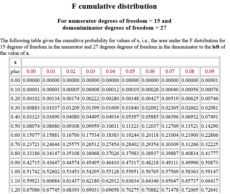 We observe that for 15 and 27 degrees of freedom P(X < 0.44) = 0.04934.
The following image shows part of the table for 27 and 15 degrees of
freedom.
Table 2
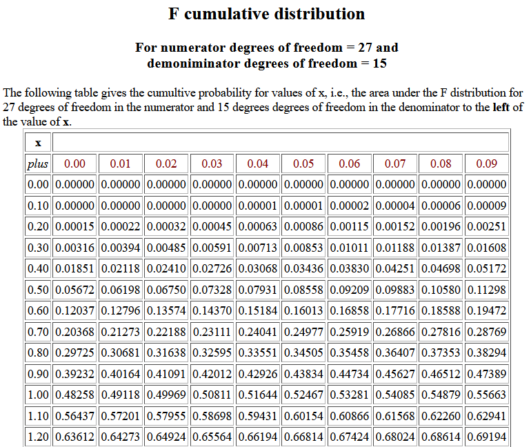 We observe that for 27 and 15 degrees of freedom P(X < 0.44) = 0.03068,
a value different from the probability seen above in Table 1.
We observe that for 27 and 15 degrees of freedom P(X < 0.44) = 0.03068,
a value different from the probability seen above in Table 1.
Here is a
link to a page that allows you to generate a specific
table for a specific pair of degrees of freedom. To
print these we would need a different table for each pair of values.
With a small enough font we might be able to squeeze each table onto
a single page. However, for numerator degrees of freedom from 1 to 100 and denominator degrees
of freedom from 1 to 100 that would take 10,000 pages. We certainly are not going to do that!
Alternatively, we could look at critical values of the F-distribution, and
then we could have a different table for each possible value of the
degrees of freedom of the numerator. Here is a
link to a page that allows you
to generate a specific table for a given numerator degrees of freedom.
To print these we would need a different table for each possible numerator value.
Each table, even with a smaller font, would take at least 7 pages to print.
Since we woud want a table for each number of numerator degrees of freedom, the whole thing
would now be down to 700 printed pages. Still way more than we are going to do as part of an appendix
to a statistics textbook.
There are two alternative ways to condense our critical value tables.
One approach is to print a separate table for each of perhaps 5 different
critical areas, say 0.001, 0.005, 0.01, 0.025, and 0.05.
Each such table might run to 4 printed pages. Therefore, we could get
the five tables in 20 printed pages.
Here is a
link to a page that allows you
to generate a specific table for a given area in the right tail.
A different approach is
to have just one table of critical values where each
row-column intersection holds four or five values, one for each of
four or five special areas.
Here is a
link to such a table.
The table shown there is really condensed. It has few choices for the degrees of freedom.
Increasing the number of those choices makes that table more useful, but also bigger.
This is the approach used in many textbooks. It usually takes up 6 to 8 pages.
A careful reading of the last two approaches reveals that they produce
tables that give critical values for specific areas to the right. What about critical values for
similar areas to the left? Would we need new tables?
Could we expand the current ones to give
critical values for areas both to the left and right?
Recall that in Table 2 above we found that
for 27 and 15 degrees of freedom P(X < 0.44) = 0.03068. Here
is a similar table that gives the cumulative probability for x
values, this time for 6 and 12 degrees of freedom.
Table 3
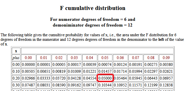 Using that table (really, reading backwards)
we can notice that P(X < 0.25) = 0.0500, that is, the value that has 0.05
area to its left is approximately 0.25. How could we get that 0.25 from the
critical value tables that we have seen so far? After all, they give the critical values for
specific areas to the right in the F distribution.
Using that table (really, reading backwards)
we can notice that P(X < 0.25) = 0.0500, that is, the value that has 0.05
area to its left is approximately 0.25. How could we get that 0.25 from the
critical value tables that we have seen so far? After all, they give the critical values for
specific areas to the right in the F distribution.
The answer may appear strange. It is a two step process.
First, we find the critical value for the
desired area to the right, but we switch the degrees of freedom. We
started with 6 and 12 degrees of freedom
(for the numerator and denominator, repectively)
so using 12 degrees of freedom for the numerator and
6 degrees of freedom for the denominator,
we use a critical value table to find the
x value that has 0.05 as the area to the right.
Look at Table 4.
Table 4
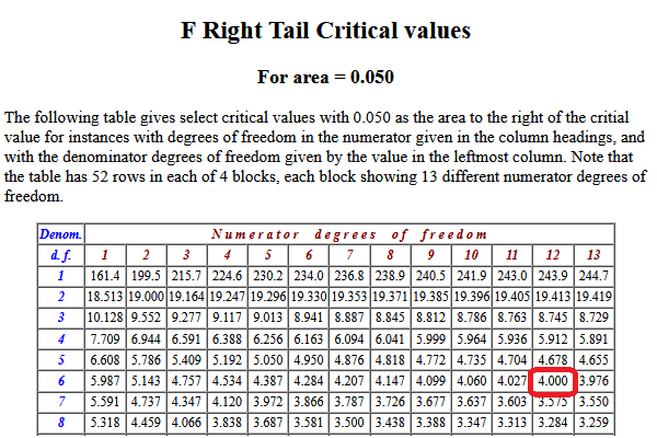 That table shows us the P( X > 4.0 ) = 0.05.
Thus, the result of our first step is the value 4.00.
That table shows us the P( X > 4.0 ) = 0.05.
Thus, the result of our first step is the value 4.00.
The second step is find the reciprocal of that value. In this case that is
1/4 which is the 0.25 that we knew from before.
This two step process was used by everyone, all the time,
along with the tables for critical values for areas to the right,
in order to find x-values that had a specifice area to the left.
Once we have access to R we no longer need tables to find
our desired values. In R we have the functions
pf() and qf().
The function pf(x,ndf,ddf) gives us the area
under the curve, for ndf degrees of freedom in the numerator
and ddf degrees of freedom in the denominator,
to the left of the value x,
i.e., the probability of getting a value less than x in the
F distribution for ndf and ddf degrees of freedom.
The function pf(x,ndf,ddf,lower.tail=FALSE) gives us the area
under the curve, for ndf degrees of freedom in the numerator
and ddf degrees of freedom in the denominator,
to the right of the value x,
i.e., the probability of getting a value greater than x in the
F distribution for ndf and ddf degrees of freedom.
The function qf(p,ndf,ddf) gives us the x-score in a
F distribution with ndf degrees of freedom in the numerator
and ddf degrees of freedom in the denominator, that has
the area under the curve to the left of x being
equal to p, i.e., that has a probability of p
of being less than x for for ndf and ddf degrees of freedom.
The function qf(p,ndf,ddf,lower.tail=FALSE) gives us the x-score in a
F distribution with ndf degrees of freedom in the numerator
and ddf degrees of freedom in the denominator, that has
the area under the curve to the right of x being
equal to p, i.e., that has a probability of p
of being greater than x for for ndf and ddf degrees of freedom.
Not that we will really use the images of the F distribution,
but it is worth seeing some of them so that we get a sense of how the
distribution depends upon the degrees of freedom and so that we can see
the changing range of the x-values.
Figure 1 shows the distribution for the degrees of freedom pair 60,60.
Figure 1
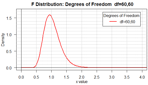
Among the many things to notice in Figure 1 are the facts that
most of the area is between x-values 0.4 and 2.0 and that the
distribution is not symmetric (note that most of the rise occurs
between 0.5 and 1 while the fall is spread out, for the most part, between
1 and 2.
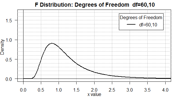
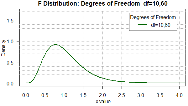
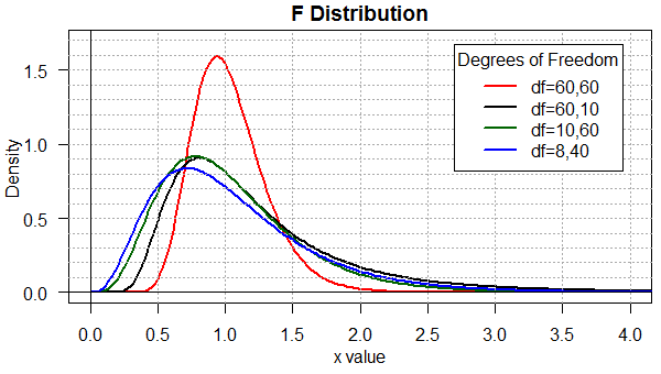
When we move to degree of freedom pairs that are not "balanced"
as in the pair 60,10 (shown in Figure 2) or the pair 10,60
(shown in Figure 3), we see a real change in the shape of the
curve.
Figure 2
| |
Figure 3
|
You should be able to see that there is a difference in the two
distributions even though the only change is to reverse the degrees of
freedom. Furthermore, in both cases, the area under the curve is
more spread out than it was in Figure 1.
Now we find appreciable area for x-values below 0.5 and above 2.0.
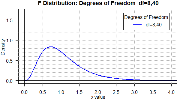
Figure 4 uses yet another degree of freedom pair. This one, 8,40,
is similar to the 10,60 we just saw in Figure 3, but, again, the graph
is noticeably different.
Figure 4
To help compare all four of the previous graphs, Figure 5
places them all on one plot.
Figure 5
Finally, toward the end of this web page you will
find the R commands used to produce these
five graphs. It is worth making a copy of those commands
and altering them appropriately to investigate other degree of freedom
pairs.
The ratio of variances
Up to this point when we want to talk about two parameters or statistics
being equal we looked at their difference and said that if they are
the same then their difference will be zero. If we have two
sample means,
45.1 and 44.8, we know that they are not identical but their difference is
small, it is close to zero.
It is either 45.1 - 44.8 = 0.3 or
44.8 - 45.1 = -0.3, values that are different only
in their sign.
Now we adopt a new approach.
For variances we know that if two variances are the same then their
ratio will be 1. If we have two sample variances, 5.1 and 4.8,
then we know that they are not equal, but their quotient is close to
1. 5.1 / 4.8 = 1.0625 and
4.8 / 5.1 ≈ 0.9412, values that are indeed close to 1.
It is important to notice that the magnitude of the difference
between each of these values and 1 is different.
Thus, when we did 5.1 / 4.8 the answer was 0.0625 away from 1.
However, when we found 4.8 / 5.1 the answer
was about 0.0588 away from 1.
Clearly, there is a difference depending upon which
value is in the numerator (the top value) and which is in the denominator
(the bottom value).
The difference that we just experienced is reflected in the
difference in the F distribution for reversed degree of freedom
pairs. When we finally start to look at
the ratio of two variances, we will want to talk about an
associated degree of freedom pair.
In that pair, the first value will be the degrees of
freedom associated with the numerator and the
second value will be the degrees of freedom associated with
the denominator. This distinction is terribly important.
|
As you might guess, the F distribution values for reversed pairs,
though different, are still related. That relation, however, at least to
novice users, is often a source of significant confusion. If time
permits, I will provide a separate page to discuss that relationship.
As it turns out, if we had to use tables then we might have to
employ that relationship. Since we have the power of R behind us,
we really have no need to use it.
|
We start with two populations that are both normal,
or at least really close to being normal.
Our interest is to find a confidence interval for the ratio of the variances of the
two populations.
We use σ1² as the variance of the first population
and σ2² as the variance of the second population.
To create a confidence interval we need to have random samples from both populations.
The samples sizes are n1
and n2, respectively.
We compute the variance of the samples.
We use s1² as the variance of the first sample
and s2² as the variance of the second sample.
We want to generate a confidence interval for the ratio of two variances.
Our first
step is to decide if we are looking at
 or
or
 .
We will get a confidence interval either way, but they will be
different confidence intervals. We just need to pick one of them.
Right now, let us choose to find the confidence
interval for .
.
We will get a confidence interval either way, but they will be
different confidence intervals. We just need to pick one of them.
Right now, let us choose to find the confidence
interval for .
Next we need to specify the level of confidence that we want.
In this example we will look at a 90% confidence interval.
That means that we want 5% of the area to the left of the confidence interval
and 5% of the area to the right.
We are looking at a 90% confidence interval for
.
From our samples we can determine
 , noting that this
quotient corresponds to the order that we had
for the population parameters,
.
The sample size of the
numerator,
, noting that this
quotient corresponds to the order that we had
for the population parameters,
.
The sample size of the
numerator,  ,
is n1.
The sample size of the
denominator,
,
is n1.
The sample size of the
denominator,  ,
is n2.
Therefore, we will use the F distribution with the degree of
freedom pair (n1-1,n2-1).
Within that distribution we want the x-value that has
5% of the area under the curve to the left of that value.
We will call this xlow.
In addition, we want the
x-value that has
5% of the area under the curve to the right of that value.
We will call this xhigh.
,
is n2.
Therefore, we will use the F distribution with the degree of
freedom pair (n1-1,n2-1).
Within that distribution we want the x-value that has
5% of the area under the curve to the left of that value.
We will call this xlow.
In addition, we want the
x-value that has
5% of the area under the curve to the right of that value.
We will call this xhigh.
The two endpoints of our confidence interval will be
(s1²/s2²)/xlow and
(s1²/s2²)/xhigh.
However, in doing this we get the endpoints in the opposite order.
For each endpoint we are dividing
s1²/s2²
by a value. Dividing that quotient by a smaller value produces a larger result
than dividing it by a larger value. Thus, the
final confidence interval will be
( (s1²/s2²)/xhigh , (s1²/s2²)/xlow).
Case 1:
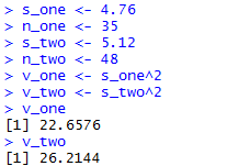
Giving numbers to the general example above, we will say that we have two samples
from two populations that are known to be normally distributed.
The first sample has size 35 and standard deviation 4.76.
The second sample has size 48 and standard deviation 5.12.
Recalling that we need to look at the variances
we find that the variance of the first sample
is 4.76² = 22.6576 and the
variance of the second sample is
5.12² = 26.2144, giving us
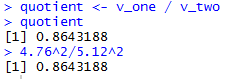
s1²/s2² ≈ 0.8643188.
We can do these computations in R
with the following commands.
s_one <- 4.76
n_one <- 35
s_two <- 5.12
n_two <- 48
v_one <- s_one^2
v_two <- s_two^2
v_one
v_two
quotient <- v_one / v_two
quotient
If we were in a hurry those commands would be needlessly long since
we could
have found that same ratio just by typing
4.76^2/5.12^2. However, we will use the longer version
so that it is easer to follow the up-coming computations.
Figure 6 shows the console view of the first 8 of those commands,
while Figure 6a shows the remaining two
along with the one statement
computation of the same quotient.
Figure 6
| |
Figure 6a
|
Because we are dealing with
s1²/s2²,
we know that the degrees of freedom
for the F distribution
will be the pair (35-1,48-1) or (34,47).
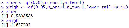
To find the x-value that has 5% of the area under the
curve of an F distribution, with 34,47 degrees of freedom,
to left of that x-value we can use the command
qf(0.05,34,47).
The result is 0.5808588, meaning that 5% of the
area under that curve is to the left of
0.5808588.
To find the x-value that has 5% of the area under the
curve of an F distribution, with 34,47 degrees of freedom,
to right of that x-value we can use the command
qf(0.05,34,47,lower.tail=FALSE).
The result is 1.677293, meaning that 5% of
the area under that curve is to the right of
1.677293. Slightly more elaborate versions of those commands
would be
xlow <- qf(0.05,n_one-1,n_two-1)
xhigh <- qf(0.05,n_one-1,n_two-1,lower.tail=FALSE)
xlow
xhigh
Figure 7 shows the R computations of those
values.
Figure 7
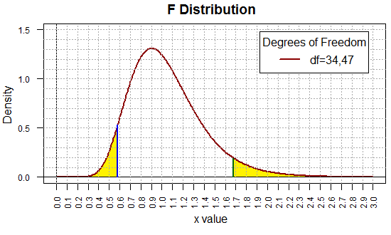
To help visualize this, Figure 8 holds the plot of the F
distribution for the degree of freedom pair (34,47). The
x-value 0.5808588 has a blue line above it and the
x-value 1.677293 has a dark green line above it.
The plot was then doctored to shade the two 5% areas in yellow.
(You might note that each of the little rectangles
in the graph represents an area
of 0.01 square units.
It is worth the moment or two to convince yourself that
the unshaded area under the curve amounts to 0.90 square units,
the 90% we sought.)
Figure 8
Of course now that we have the xlow and xhigh
values we still have the final computation to do to generate
our confidence interval. That computation amounts to finding
(s1²/s2²)/xhigh and
(s1²/s2²)/xlow.
We can do this in R via the commands
c_low <- quotient/xhigh
c_high <- quotient/xlow
c_low
c_high
remembering that to get the low end of the confidence interval
we divide that quotient by the larger value, xhigh, whereas to get the
upper end of the confidence interval we divide the
quotient by the smaller value, xlow.
Figure 9 shows the result of those commands.
Figure 9
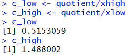
Thus, our 90% confidence interval for the
ratio of the population variances,
,
is (0.515,1.488).
Case 1 (revisited):
Rather than just jumping into a completely new
example, we will redo the previous case, but this time we
look at the inverse ratio.
That is, we
will look for the 90% confidence interval for the
ratio of .
I can see three ways to approach this new problem.
The first is to use the values assigned above in Figure 6.
Then we could redo the commands shown in Figures 6a,
swapping the placement of v_one and v_two,
as well as the commands in Figure 7
swapping the placement of n_one and n_two.
The computation in Figure 9 stays the same.
Thus the sequence of commands would be
# now do it over, swapping variables
s_one <- 4.76
n_one <- 35
s_two <- 5.12
n_two <- 48
v_one <- s_one^2
v_two <- s_two^2
v_one
v_two
quotient <- v_two / v_one
xlow <- qf(0.05,n_two-1,n_one-1)
xhigh <- qf(0.05,n_two-1,n_one-1,lower.tail=FALSE)
xlow
xhigh
c_low <- quotient/xhigh
c_high <- quotient/xlow
c_low
c_high
The console view of those commands is given in Figure 10
and Figure 10a.
Figure 10
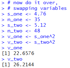
| |
Figure 10a
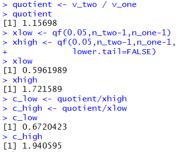
|
As you can see we have a new ratio, 1.15698,
new low and high F values,
0.5962989 and 1.721589
(because the order of the degree of freedom values has changed),
and a new confidence interval (0.672,1.94).
A second approach to solving this new case would have been
to just swap the original values. Yes, we want to find
the confidence interval for
,
and yes the original statements found the
confidence interval for
,
but the original associated n_one and s_one
with the values for
 .
Why not leave the commands as they were
and just associate n_one and s_one
with
.
Why not leave the commands as they were
and just associate n_one and s_one
with  ,
and associate
n_two and s_two
with ?
Doing that would produce the sequence of commands
,
and associate
n_two and s_two
with ?
Doing that would produce the sequence of commands
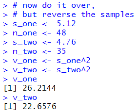
# now do it over,
# but reverse the samples
s_one <- 5.12
n_one <- 48
s_two <- 4.76
n_two <- 35
v_one <- s_one^2
v_two <- s_two^2
v_one
v_two
quotient <- v_one / v_two
quotient
xlow <- qf(0.05,n_one-1,n_two-1)
xhigh <- qf(0.05,n_one-1,n_two-1,
            lower.tail=FALSE)
xlow
xhigh
c_low <- quotient/xhigh
c_high <- quotient/xlow
c_low
c_high
Figure 11
| |
Figure 11a

|
Of course, we get the same results
in Figure 11a as we did in Figure 10a.
The first approach had us changing the real computational commands
while the second had us changing the association of values to variables.
Both are somewhat confusing. Here is a third approach.
Change the commands, once and for all,
to use variables that are just associated with the
top or bottom variance rather than being associated with a
numbered, 1 or 2, variance. Now
the commands appear as
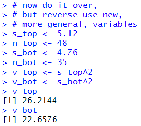
# now do it over,
# but reverse use new,
# more general, variables
s_top <- 5.12
n_top <- 48
s_bot <- 4.76
n_bot <- 35
v_top <- s_top^2
v_bot <- s_bot^2
v_top
v_bot
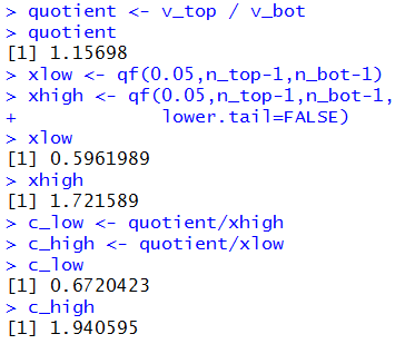
quotient <- v_top / v_bot
quotient
xlow <- qf(0.05,n_top-1,n_bot-1)
xhigh <- qf(0.05,n_top-1,n_bot-1,
lower.tail=FALSE)
xlow
xhigh
c_low <- quotient/xhigh
c_high <- quotient/xlow
c_low
c_high
Figure 12 and 12a show the console view of those commands.
Figure 12
| |
Figure 12a
|
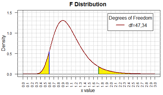
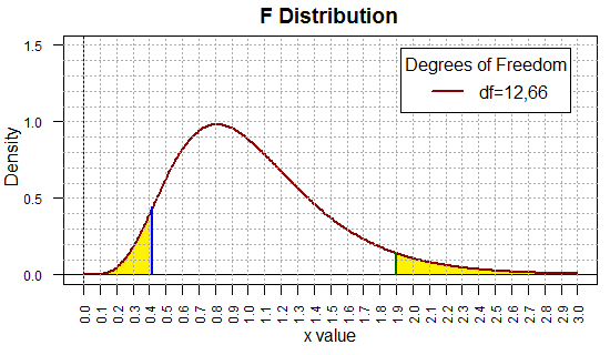
Before we leave this case, we should at least look at the appropriate
F distribution, noting the cutoff points that we found in
Figure 12a, namely, 0.5961989 and 1.721589.
The plot of that F distribution is given in Figure 13.
As in Figure 8, this image has been doctored to show the two 5%
regions in yellow.
Figure 13
The beauty of this new set of commands, given above Figure 12,
is that
we can apply it, logically, to any new problem.
For example, if we have two normal populations,
one of Ford products and one of General Motors products,
and we want to get a 90% confidence interval
for the quotient of the variance of the GM products to the
variance of the Ford products, then we can take two random samples
and get their sample size and sample standard deviation.
Then, we plug in the GM values for the top variables
and the Ford sample values for the bot variables
and all of the rest of the computations stay the same.
Case 2: We have such a case. The Ford sample is of size 67
with standard deviation of 14.27 while
the GM sample is of size 13 with sample
standard deviation of 11.34. We know that the
GM values are to be associated with the top
variables. Thus, our commands become
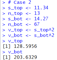
# Case 2
s_top <- 11.34
n_top <- 13
s_bot <- 14.27
n_bot <- 67
v_top <- s_top^2
v_bot <- s_bot^2
v_top
v_bot
quotient <- v_top / v_bot
quotient
xlow <- qf(0.05,n_top-1,n_bot-1)
xhigh <- qf(0.05,n_top-1,n_bot-1,
            lower.tail=FALSE)
xlow
xhigh
c_low <- quotient/xhigh
c_high <- quotient/xlow
c_low
c_high
They produce the console views shown in Figure 14 and Figure 14a.
Figure 14
| |
Figure 14a

|
Therefore, our 90% confidence interval for the ratio of the GM variance to
the Ford variance is
(0.332,1.501). While we are at it,
Figure 15 shows the marked-up
F distribution that we would be using for this problem.
Figure 15
Although it is nice to have this general set of commands to do
our work, it would be even nicer to capture them in a function.
When we do this we will want to add a specification for the
confidence level.
Consider the following function definition:
ci_2popvar <- function (
             n_top, s_top, n_bot, s_bot,
             cl=0.95)
{ # generate a confidence interval for the  ratio
  # of the top variance to the bottom variance from
  # a sample of the top population with size n_top
  # and standard deviation s_top and a sample of the
  # bottom population with size n_bot and standard
  # deviation s_bot.  cl gives the confidence level.

alpha <- 1-cl
alphadiv2 <- alpha/2
v_top <- s_top^2
v_bot <- s_bot^2
quotient <- v_top / v_bot
xlow <-  qf( alphadiv2, n_top-1,n_bot-1)
xhigh <- qf( alphadiv2, n_top-1,n_bot-1,
            lower.tail=FALSE)
c_low <- quotient/xhigh
c_high <- quotient/xlow

result <- c( c_low, c_high, quotient,
             xlow, xhigh, v_top,
             s_top, n_top, v_bot, s_bot,
             n_bot, cl, alphadiv2)
names(result) <-
          c( "CI Low", "CI_HIGH", "Quotient",
             "F Low",  "F High",  "Top Var.",
             "Top sd", "Top size", "Bot Var.",
             "Bot sd", "Bot size", "C level",
             "Alpha/2")
return( result)
}
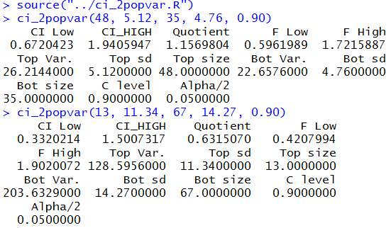
With that function placed in the parent directory we can
use the commands
source("../ci_2popvar.R")
ci_2popvar(48, 5.12, 35, 4.76, 0.90)
ci_2popvar(13, 11.34, 67, 14.27, 0.90)
to do all of the work in Figures 12, 12a, 14, and 14a.
The results are shown in Figure 16.
Figure 16
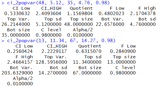
Then, too, with a simple change we can do that same work again, but this time to
get a 98% confidence interval.
Those commands would be
ci_2popvar(48, 5.12, 35, 4.76, 0.98)
ci_2popvar(13, 11.34, 67, 14.27, 0.98)
and their results are shown in Figure 17.
Figure 17
Hypothesis test
Having worked our way through the construction of confidence intervals
our next challenge is to construct a test for the null hypothesis
that two populations, known to be normal, have the same variance.
That is, we want to have a test for
H0: σ1² = σ2².
As we have seen before, we will have to have an alternative
hypothesis and it will take the form of one of
-
H1: σ1² ≠ σ2².
-
H1: σ1² < σ2².
-
H1: σ1² > σ2².
To do this test we will take two samples, one from each population, and
we will find the variance of each sample. If the null hypothesis is true
then we expect that the two sample variances will be approximately equal.
Evidence to indicate that the null hypothesis is not true would be to find
that the sample variance differs significantly.
In earlier hypothesis tests we looked for such evidence by finding
the difference of the sample statistics.
We did that because we knew, in those earlier situations,
the distribution of the difference of the sample statistics.
Here we know the distribution of the ratio of the sample statistics,
that is, we know that
s1² / s2²
is a F distribution with the degree of freedom pair
(n1-1, n2-1).
Using this we can restate the null
hypothesis as
H0: σ1² / σ2² = 1.
and the alternative hypotheses as
-
H1: σ1² / σ2² ≠ 1.
-
H1: σ1² / σ2² < 1.
-
H1: σ1² / σ2² > 1.
To reject H0 in favor of
H1: σ1² / σ2² ≠ 1.
we will need to have the value of
s1² / s2²
be far enough away, in either direction, from 1 that the probability
of getting that kind of value will be less than the stated level of significance.
To reject H0 in favor of
H1: σ1² / σ2² < 1.
we will need to have the value of
s1² / s2²
be far enough away, toward 0, from 1, that the probability
of getting that kind of value will be less than the stated level of significance.
To reject H0 in favor of
H1: σ1² / σ2² > 1.
we will need to have the value of
s1² / s2²
be far enough away, above 1, from 1, that the probability
of getting that kind of value will be less than the stated level of significance.
Let us try a few examples.
Case 3: We have two populations, both known to be normal and we want to test
H0: σ1² / σ2² = 1.
against the alternative hypothesis
H1: σ1² / σ2² ≠ 1.
at the 0.05 level of significance. We take samples from the two
populations. The sample from the first population is of size 36 and it has a sample standard
deviation of 23.14, therefore the sample variance is 23.14² or 535.4596.
The sample from the second population is of size 58 and it has a sample standard
deviation of 28.31, therefore the sample variance is 28.31² or 801.4561.
The quotient of the variances will be 535.4596 / 801.4561 which is
about 0.6681.
The ratio of the variances will have a F distribution
with the degree of freedom pair (35,57).
Since this is a 2-sided test, for that degree of freedom pair we want the x-value
that has 0.025 of the area to its left and the
x-value that has 0.025 of the area to its right.
Those values are 0.535 and 1.7888, respectively.
These are our critical values. But our quotient was 0.6681 and this
is not outside of our critical values so we say that we do not have
sufficient evidence to reject H0.
For the attained significance approach, we need to find the probability
of getting a ratio more extreme than 0.6681. This ratio is less than 1 so we want
to find the area under the F-distribution with
35 and 57 degrees of freedom to the left of 0.6681.
Once we get that value, we need to double it to account for upper tail.
The left-tail value is about 0.10176.
Therefore, our attained significance would be 0.20352 a value
that is not less than the specified level of significance, 0.05, so we say that
we do not have sufficient evidence to reject H0.
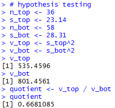
The R statements to do these calculations could be:
# hypothesis testing
n_top <- 36
s_top <- 23.14
n_bot <- 58
s_bot <- 28.31
v_top <- s_top^2
v_bot <- s_bot^2
v_top
v_bot
quotient <- v_top / v_bot
quotient
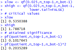
xlow <- qf(0.025,n_top-1,n_bot-1)
xhigh <- qf(0.025,n_top-1,n_bot-1,
lower.tail=FALSE)
# critical values
xlow
xhigh
# attained significance
pf(quotient,n_top-1,n_bot-1)
pf(quotient,n_top-1,n_bot-1)*2
The console view of those statements is
shown in Figure 18 and Figure 18a.
Figure 18
| |
Figure 18a
|
Case 3 (reversed): For this case we use exactly the same values
as in the previous case but we will reverse the populations. That is,
instead of looking at the ratio
H0: σ1² / σ2² = 1
we will look at the ratio
H0: σ2² / σ1² = 1.
The alternative hypothesis is now
H1: σ2² / σ1² ≠ 1.
We have the same samples, so they have the same variances.
However, this time we will look at the sample
statistic
s2² / s1².
Again, in order to reject H0 the particular value of that
sample statistic will have to be sufficiently far from 1.
The distribution of such a sample statistic is a F distribution with
(58-1,36-1) degrees of freedom. It is important to note that
we had to reverse the order of those
values because the top (numerator) of the ratio
s2² / s1²
is the s2 and the first of the pair
of the degrees of freedom is associated with the top (numerator) value
in the quotient. Of course, that change means that we have to again find
the x-value in the F distribution with (57,35) degrees
of freedom that has 2.5% of the area to its left and we
need to find the similar value that has 2.5% of the area to its right.
These values, which are different from the ones we
found above because the degrees of freedom changed,
are 0.559 and 1.869, respectively.
These are the critical values.
When we calculate the ratio 801.4561 / 535.4596 we get
1.497, and this is not extreme enough to reject the null hypothesis
in favor of the alternative at the 0.05 level of significance.
We could have used the attained significance approach and
looked at how "strange" is it to get the ratio 1.497 if
the null hypothesis is true. Since that ratio is greater than 1
we need to look at the probability of getting that value or higher
if H0 is true. That probability
turns out to be 0.10176. Of course, since this is a two-tail
test we need to double that to account for being "that far" off in the other
direction. Therefore, the attained significance is, again,
0.20352, a value that is not less than the level of
significance specified, 0.05, so we do not have sufficient
evidence to reject the null hypothesis in favor of the alternative
hypothesis. You might have noticed that this attained significance
is exactly the same as the attained significance in the original Case 3
example. There, with (35,57) degrees of freedom we looked at the
left tail and then doubled it, here with (57,35) degrees of freedom, we looked
at the right tail and then doubled it.
With those correct interpretations we certainly should get the
same attained significance for the samples that we have.
Other than changing the computation of the attained significance
to use the upper tail,
and of course changing the initial assignments of values,
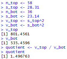
the R statements remain the same.
n_top <- 58
s_top <- 28.31
n_bot <- 36
s_bot <- 23.14
v_top <- s_top^2
v_bot <- s_bot^2
v_top
v_bot
quotient <- v_top / v_bot
quotient
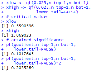
xlow <- qf(0.025,n_top-1,n_bot-1)
xhigh <- qf(0.025,n_top-1,n_bot-1,
lower.tail=FALSE)
# critical values
xlow
xhigh
# attained significance
pf(quotient,n_top-1,n_bot-1,
lower.tail=FALSE)
pf(quotient,n_top-1,n_bot-1,
lower.tail=FALSE)*2
The console view of those statements is given in
Figure 19 and Figure 19a.
Figure 19
| |
Figure 19a
|
Case 4:We have two normally distributed populations.
We want to test the hypothesis that they have equal variances
against the alternative that the variance of the first is greater than
the variance of the second.
We note that if the first is greater than the second then
the first divided by the second will be greater than 1.
We want to run this test at the 0.01 level of significance.
We take two samples and find that the sample from the first
population is of size 87 and it has a sample standard deviation
of 32.19 while the sample from the second population is of size 43
and it has a standard deviation of 48.52.
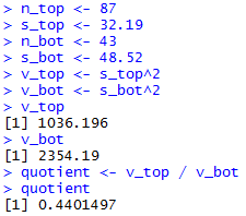
From this information we see that the first sample variance
is 1036.196 and the second sample variance is 2354.19,
giving us the ratio 0.44.
We can stop our analysis right there. The alternative is that the
first variance is greater than the second, equivalently that the ratio of
the first to the second is greater than 1. To reject the null hypothesis,
we need to have the samples give us a ratio that is significantly larger
than 1. The samples that we have yield a ratio that is less than 1.
This is certainly no evidence that we should reject
H0 in favor
of H1.
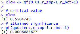
Of course we could find the critical value.
We are looking for the x-value for the
F distribution curve with the degree of freedom pair (86,42) that
has 1% of the area to its right. That turns out to be
about 1.9317.
We would have enough evidence to reject H0
if the sample statistic is greater than the critical value.
Clearly, 0.44 is not greater than 1.9317. We do not have evidence to reject
H0 in favor of the alternative.
The attained significance of our absurdly low ratio is
0.999 which is clearly not less than the 0.01 significance
level of the test.
The R commands that produced those values follow.
# case 4
n_top <- 87
s_top <- 32.19
n_bot <- 43
s_bot <- 48.52
v_top <- s_top^2
v_bot <- s_bot^2
v_top
v_bot
quotient <- v_top / v_bot
quotient

xhigh <- qf(0.01,n_top-1,n_bot-1,
            lower.tail=FALSE)
# critical value
xhigh
# attained significance
pf(quotient,n_top-1,n_bot-1,
   lower.tail=FALSE)
Case 5: For this example we will repeat
the previous one but with a different
alternative hypothesis. Now
H1: σ1² / σ2² < 1.
With this as the alternative we need to have
the ratio of the sample variances be far below 1 in order
to reject the null hypothesis.
How far below 1 do we need to be?
The x-value in the F distribution with the degrees of freedom
pair (86,42) that has 1% of the area to its left is
0.5504748. Thus, our one critical value
for this one-tail test is 0.5504748.
The ratio of the variances is
1036.196 / 2354.19 ≈ 0.44, a value that is
even further away from 1 than is the critical value.
Therefore, our samples give us sufficient evidence to reject
H0 in favor of
H1 at the 0.01 level of significance.
The R statements for those computations follow.
n_top <- 87
s_top <- 32.19
n_bot <- 43
s_bot <- 48.52
v_top <- s_top^2
v_bot <- s_bot^2
v_top
v_bot
quotient <- v_top / v_bot
quotient

xlow <- qf(0.01,n_top-1,n_bot-1)

# critical value
xlow
# attained significance
pf(quotient,n_top-1,n_bot-1)
The console view of the statements is given in Figure 20
and Figure 20a.
Figure 20
| |
Figure 20a
|
We have seen that pretty much the same statements
are used to solve all of our problems. We want to capture these in
a function. Here is one such function.
hypoth_2test_var <- function(
       n_top, s_top, n_bot, s_bot,
       H1_type, sig_level=0.05)
{ # perform a hypothsis test for equality of
  # the variances of two populations
  # based on two samples of n_top and n_not
  # items yielding sample
  # standard deviations s_top and s_bot
  #  where the alternative hypothesis  is
  #      !=  if H1_type==0
  #      <   if H1_type < 0
  #      >   if H1_type > 0
  # Do the test at sig_level significance,
  #
  # It is important that the population is a normal
  # distribution.

  decision <- "do not reject"
  v_top = s_top^2
  v_bot = s_bot^2
  quotient <- v_top / v_bot
  alpha <- sig_level
  if ( H1_type == 0 )
     { alpha <- alpha/2 }
  #find the critical value(s)
  xlow <- qf(alpha,n_top-1,n_bot-1)
  xhigh <- qf( alpha, n_top-1, n_bot-1,
               lower.tail=FALSE)
  if( H1_type == 0 )
    {  if( (quotient < xlow) | (quotient>xhigh) )
         { decision <- "Reject" }
       if (quotient < 1 )
         { attained = 2*pf(quotient,n_top-1,n_bot-1)}
         else
         { attained = 2*pf(quotient, n_top-1,
                          n_bot-1, lower.tail=FALSE) }
       H1 <- "v_1 != v_2"
    }
    else if( H1_type < 0 )
    {  if( quotient < xlow )
         { decision <- "Reject" }
       attained = pf( quotient,n_top-1,n_bot-1)
       xhigh <- "n.a."
       H1 <- "v_1 < v_2"
    }
    else
    {  if( quotient > xhigh )
         { decision <- "Reject" }
       attained = pf( quotient,n_top-1,
                n_bot-1,lower.tail=FALSE)
       xlow <- "n.a."
       H1 <- "v_1 > v_2"
    }
   result <- c( H1, n_top, s_top, v_top,
             n_bot, s_bot, v_bot, quotient, xlow,
             xhigh, decision, attained )
   names(result) <- c( "H1","n top", "s top", "v top",
              "n bot", "s bot", "v bot",
              "quotient", "crit low", "crit high",
              "decision", "attained")
   return (result)
  }
Then, assuming we have placed the source code for that
function in a file named hypo_2var.R in the parent
directory (folder), we could load the function
and do all four of the tests above via the statements
source("../hypo_2var.R")
#case 3
hypoth_2test_var( 36, 23.14, 58, 28.31, 0, 0.05)
#case 3 reversed
hypoth_2test_var( 58, 28.31, 36, 23.14, 0, 0.05)
#case 4
hypoth_2test_var(87, 32.19, 43, 48.52, 1, 0.01)
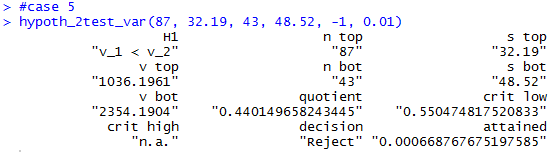
#case 5
hypoth_2test_var(87, 32.19, 43, 48.52, -1, 0.01)
The console view of those is given in Figures 21 through 24.
Figure 21
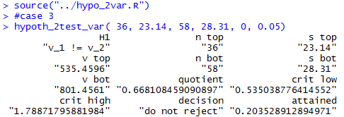
Figure 22
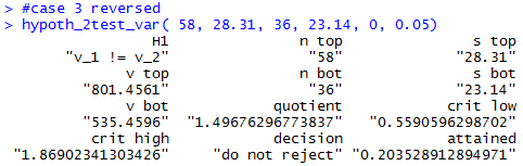
Figure 23
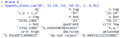
Figure 24
Below is a listing of the R commands used
in generating plots in Figures 1 through 5 above.
# Display the F distributions with
# four different sets of pairs of degrees of freedom.

x <- seq(0, 4.5, length=200)
hx <- rep(0,200)

degf1 <- c(60,60,10,8)
degf2 <- c(60,10,60,40)
colors <-  c("red",  "black", "darkgreen", "blue")
labels <- c("df=60,60",  "df=60,10",  "df=10,60",  "df=8,40")


plot(x, hx, type="n", lty=2, lwd=2, xlab="x value",
     ylab="Density", ylim=c(0,1.7), xlim=c(0,4), las=1,
     xaxp=c(0,4,8),
     main="F Distribution "
     )

for (i in 1:4){
  lines(x, df(x,degf1[i],degf2[i]), lwd=2, col=colors[i], lty=1)
}
abline(h=0)
abline(h=seq(0.1,1.7,0.1), lty=3, col="darkgray")
abline(v=0)
abline(v=seq(0.5,4,0.5), lty=3, col="darkgray")
legend("topright", inset=.05, title="Degrees of Freedom",
       labels, lwd=2, lty=1, col=colors)


for (j in 1:4 ){
plot(x, hx, type="n", lty=2, lwd=2, xlab="x value",
     ylab="Density", ylim=c(0,1.7), xlim=c(0,4), las=1,
     xaxp=c(0,4,8),
     main=paste("F Distribution: Degrees of Freedom ",labels[j])
     )

for (i in j:j){
  lines(x, df(x,degf1[i],degf2[i]), lwd=2, col=colors[i], lty=1)
}
abline(h=0)
abline(h=seq(0.1,1.7,0.1), lty=3, col="darkgray")
abline(v=0)
abline(v=seq(0.5,4,0.5), lty=3, col="darkgray")
legend("topright", inset=.05, title="Degrees of Freedom",
       labels[j], lwd=2, lty=1, col=colors[j])

}
Here is a listing of the computational commands used in creating
this page:
s_one <- 4.76
n_one <- 35
s_two <- 5.12
n_two <- 48
v_one <- s_one^2
v_two <- s_two^2
v_one
v_two
quotient <- v_one / v_two
quotient
4.76^2/5.12^2

xlow <- qf(0.05,n_one-1,n_two-1)
xhigh <- qf(0.05,n_one-1,n_two-1,lower.tail=FALSE)
xlow
xhigh

x <- seq(0, 3, length=300)
hx <- rep(0,300)
degf1 <- n_one - 1
degf2 <- n_two - 1
colors <- "darkred"
labels <- paste("df=",n_one-1,",",n_two-1,sep="")
plot(x, hx, type="n", lty=2, lwd=2, xlab="x value",
     ylab="Density", ylim=c(0,1.5), xlim=c(0,3), las=2,
     xaxp=c(0,3,30),cex.axis=0.75,
     main="F Distribution "
     )
lines(x, df(x,degf1,degf2), lwd=2, col=colors, lty=1)
abline(h=0)
abline(h=seq(0.1,1.5,0.1), lty=3, col="darkgray")
abline(v=0)
abline(v=seq(0.0,3,0.1), lty=3, col="darkgray")
legend("topright", inset=.05, title="Degrees of Freedom",
       labels, lwd=2, lty=1, col=colors)
lines(c(xlow,xlow),c(0,df(xlow,degf1,degf2)),col="blue",lw=2)
lines(c(xhigh,xhigh),c(0,df(xhigh,degf1,degf2)),col="darkgreen",lw=2)

c_low <- quotient/xhigh
c_high <- quotient/xlow
c_low
c_high

# now do it over,
# swapping variables
s_one <- 4.76
n_one <- 35
s_two <- 5.12
n_two <- 48
v_one <- s_one^2
v_two <- s_two^2
v_one
v_two
quotient <- v_two / v_one
quotient
xlow <- qf(0.05,n_two-1,n_one-1)
xhigh <- qf(0.05,n_two-1,n_one-1,
            lower.tail=FALSE)
xlow
xhigh
c_low <- quotient/xhigh
c_high <- quotient/xlow
c_low
c_high

# now do it over,
# but reverse the samples
s_one <- 5.12
n_one <- 48
s_two <- 4.76
n_two <- 35
v_one <- s_one^2
v_two <- s_two^2
v_one
v_two
quotient <- v_one / v_two
quotient
xlow <- qf(0.05,n_one-1,n_two-1)
xhigh <- qf(0.05,n_one-1,n_two-1,
            lower.tail=FALSE)
xlow
xhigh
c_low <- quotient/xhigh
c_high <- quotient/xlow
c_low
c_high

# now do it over,
# but reverse use new,
# more general, variables
s_top <- 5.12
n_top <- 48
s_bot <- 4.76
n_bot <- 35
v_top <- s_top^2
v_bot <- s_bot^2
v_top
v_bot
quotient <- v_top / v_bot
quotient
xlow <- qf(0.05,n_top-1,n_bot-1)
xhigh <- qf(0.05,n_top-1,n_bot-1,
            lower.tail=FALSE)
xlow
xhigh
c_low <- quotient/xhigh
c_high <- quotient/xlow
c_low
c_high


x <- seq(0, 3, length=300)
hx <- rep(0,300)
degf_top <- n_top - 1
degf_bot <- n_bot - 1
colors <- "darkred"
labels <- paste("df=",n_top-1,",",n_bot-1,sep="")
plot(x, hx, type="n", lty=2, lwd=2, xlab="x value",
     ylab="Density", ylim=c(0,1.5), xlim=c(0,3), las=2,
     xaxp=c(0,3,30),cex.axis=0.75,
     main="F Distribution "
     )
lines(x, df(x,degf_top,degf_bot), lwd=2, col=colors, lty=1)
abline(h=0)
abline(h=seq(0.1,1.5,0.1), lty=3, col="darkgray")
abline(v=0)
abline(v=seq(0.0,3,0.1), lty=3, col="darkgray")
legend("topright", inset=.05, title="Degrees of Freedom",
       labels, lwd=2, lty=1, col=colors)
lines(c(xlow,xlow),c(0,df(xlow,degf_top,degf_bot)),col="blue",lw=2)
lines(c(xhigh,xhigh),c(0,df(xhigh,degf_top,degf_bot)),col="darkgreen",lw=2)


# Case 2
s_top <- 11.34
n_top <- 13
s_bot <- 14.27
n_bot <- 67
v_top <- s_top^2
v_bot <- s_bot^2
v_top
v_bot
quotient <- v_top / v_bot
quotient
xlow <- qf(0.05,n_top-1,n_bot-1)
xhigh <- qf(0.05,n_top-1,n_bot-1,
            lower.tail=FALSE)
xlow
xhigh
c_low <- quotient/xhigh
c_high <- quotient/xlow
c_low
c_high

x <- seq(0, 3, length=300)
hx <- rep(0,300)
degf_top <- n_top - 1
degf_bot <- n_bot - 1
colors <- "darkred"
labels <- paste("df=",n_top-1,",",n_bot-1,sep="")
plot(x, hx, type="n", lty=2, lwd=2, xlab="x value",
     ylab="Density", ylim=c(0,1.5), xlim=c(0,3), las=2,
     xaxp=c(0,3,30),cex.axis=0.75,
     main="F Distribution "
     )
lines(x, df(x,degf_top,degf_bot), lwd=2, col=colors, lty=1)
abline(h=0)
abline(h=seq(0.1,1.5,0.1), lty=3, col="darkgray")
abline(v=0)
abline(v=seq(0.0,3,0.1), lty=3, col="darkgray")
legend("topright", inset=.05, title="Degrees of Freedom",
       labels, lwd=2, lty=1, col=colors)
lines(c(xlow,xlow),c(0,df(xlow,degf_top,degf_bot)),col="blue",lw=2)
lines(c(xhigh,xhigh),c(0,df(xhigh,degf_top,degf_bot)),col="darkgreen",lw=2)

source("../ci_2popvar.R")
ci_2popvar(48, 5.12, 35, 4.76, 0.90)
ci_2popvar(13, 11.34, 67, 14.27, 0.90)
#
ci_2popvar(48, 5.12, 35, 4.76, 0.98)
ci_2popvar(13, 11.34, 67, 14.27, 0.98)
#

# hypothesis testing
n_top <- 36
s_top <- 23.14
n_bot <- 58
s_bot <- 28.31
v_top <- s_top^2
v_bot <- s_bot^2
v_top
v_bot
quotient <- v_top / v_bot
quotient
xlow <- qf(0.025,n_top-1,n_bot-1)
xhigh <- qf(0.025,n_top-1,n_bot-1,
            lower.tail=FALSE)
# critical values
xlow
xhigh
# attained significance
pf(quotient,n_top-1,n_bot-1)
pf(quotient,n_top-1,n_bot-1)*2

# redo the example but reverse the
# ratio, so degrees of freedom
# reverse
n_top <- 58
s_top <- 28.31
n_bot <- 36
s_bot <- 23.14
v_top <- s_top^2
v_bot <- s_bot^2
v_top
v_bot
quotient <- v_top / v_bot
quotient

xlow <- qf(0.025,n_top-1,n_bot-1)
xhigh <- qf(0.025,n_top-1,n_bot-1,
            lower.tail=FALSE)
# critical values
xlow
xhigh
# attained significance
pf(quotient,n_top-1,n_bot-1,
   lower.tail=FALSE)
pf(quotient,n_top-1,n_bot-1,
   lower.tail=FALSE)*2

# case 4
n_top <- 87
s_top <- 32.19
n_bot <- 43
s_bot <- 48.52
v_top <- s_top^2
v_bot <- s_bot^2
v_top
v_bot
quotient <- v_top / v_bot
quotient

xhigh <- qf(0.01,n_top-1,n_bot-1,
            lower.tail=FALSE)
# critical value
xhigh
# attained significance
pf(quotient,n_top-1,n_bot-1,
   lower.tail=FALSE)


# case 5
n_top <- 87
s_top <- 32.19
n_bot <- 43
s_bot <- 48.52
v_top <- s_top^2
v_bot <- s_bot^2
v_top
v_bot
quotient <- v_top / v_bot
quotient

xlow <- qf(0.01,n_top-1,n_bot-1)

# critical value
xlow
# attained significance
pf(quotient,n_top-1,n_bot-1)


# define our function

source("../hypo_2var.R")
#case 3
hypoth_2test_var( 36, 23.14, 58, 28.31, 0, 0.05)
#case 3 reversed
hypoth_2test_var( 58, 28.31, 36, 23.14, 0, 0.05)
#case 4
hypoth_2test_var(87, 32.19, 43, 48.52, 1, 0.01)
#case 5
hypoth_2test_var(87, 32.19, 43, 48.52, -1, 0.01)
Return to Topics page
©Roger M. Palay
Saline, MI 48176 April, 2026