Two Populations; Proportions

Return to Topics page
This is a situation where we have two populations. Furthermore, within those populations we can distinguish characteristics such that we can say that the proportion of population 1 that has a specific characteristic is p₁ and the proportion of population 2 that has the same characteristic is p₂. We are interested in the difference of those proportions, that is, p₁ - p₂.

We will start, as we have for other situations, by looking at the process that we need to use to create a confidence interval, at some level of confidence, for the difference of two proportions. Later we will look at the process that we need to use to test the null hypothesis, at some significance level, that the difference of the two proportions is zero. That translates to having the null hypothesis state that the two proportions are equal.

The confidence interval for the difference of two proportions

We create the confidence interval for the difference of two proportions from two samples, one from each population. We can recognize that the samples are of size n₁ and n₂. Each sample will have a number of its items that have the specified characteristic for that population. We will say that x₁ is the number of items in the first sample that exhibit the characteristic of population one. In the same way, we will say that x₂ is the number of items in the second sample that exhibit the characteristic of population two.

Using those values we see that we have

and

. Then

is an estimate of p₁,

is an estimate of p₂, and

is an estimate of p₁ - p₂.

For our confidence interval we need a point estimate of p₁ - p₂ and we have that in

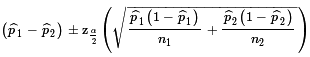
. Then we need to know the distribution of the point estimate. Under certain conditions we can consider

to be normal with mean p₁ - p₂ and standard deviation, called the standard error,

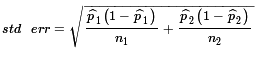. The required conditions are

These are random samples
The samples are independent
The samples are big enough to have at least 10 successes and 10 failures in each sample
The samples are small enough so that they represent less than 5% of their respective populations.

Of course, in any particular problem, we will need to specify the confidence level. For a 95% confidence level we will want to allow the remaining 5% to fall outside of the confidence interval. Because this is a normal distribution it is symmetric. If we let α represent that outside 5%, then want z_α/2 to be either the value in the standard normal distribution that has α/2 of the area below it or α/2 of the area above it.

With all of that we have the confidence interval specified as (point estimate) ± z_α/2 * std err
or

Case 1: We have two large populations and they each exhibit characteristics that we will call "successes" and "failures". We have a random sample of size 66 from population 1, of which 43 are successes, thus there are 23 failures in this sample. We have a random sample of size 87 from population 2, of which 68 are successes, thus there are 19 failures in this sample. We want to construct a 95% confidence interval for the difference in the population proportions, p₁ - p₂.

Our computations become

= 43/66 ≈ 0.6515

= 68/87 ≈ 0.7816

≈ 0.6515 - 0.7816 = -0.1301
α = 1-0.95 = 0.05
α/2 = 0.025
z_α/2 ≈ -1.96

≈

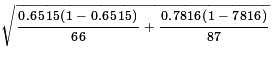≈ 0.735
margin of error = z_α/2 * std err ≈ -1.96 * 0.735 ≈ -0.144
interval = ± moe ≈ -0.1301 ± -0.144 ≈ (-0.2741, 0.0139)

Of course we could do these calculations in R via the commands

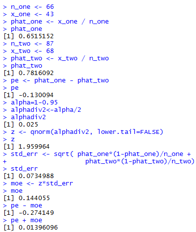
n_one <- 66
x_one <- 43
phat_one <- x_one / n_one
phat_one
n_two <- 87
x_two <- 68
phat_two <- x_two / n_two
phat_two
pe <- phat_one - phat_two
pe
alpha=1-0.95
alphadiv2<-alpha/2
alphadiv2
z <- qnorm(alphadiv2, lower.tail=FALSE)
z
std_err <- sqrt( phat_one*(1-phat_one)/n_one +
                   phat_two*(1-phat_two)/n_two)
std_err
moe <- z*std_err
moe
pe - moe
pe + moe

Figure 1 gives the console view of these commands.

Figure 1

The pattern for finding such a confidence interval does not change. About the only wrinkle that might be added is to start with the raw data.

Case 2: Consider the data in Table 1 and in Table 2. In those tables a success is an item with the value 2, anything else is a failure.

Assuming that Table 1 and Table 2 represent random samples from two populations that have more than 1480 and 1780 members respectively, we can create a 90% confidence interval via the computations

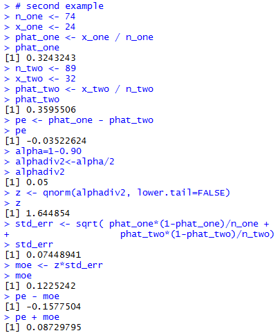
# second example
n_one <- 74
x_one <- 24
phat_one <- x_one / n_one
phat_one
n_two <- 89
x_two <- 32
phat_two <- x_two / n_two
phat_two
pe <- phat_one - phat_two
pe
alpha=1-0.90
alphadiv2<-alpha/2
alphadiv2
z <- qnorm(alphadiv2, lower.tail=FALSE)
z
std_err <- sqrt( phat_one*(1-phat_one)/n_one +
                   phat_two*(1-phat_two)/n_two)
std_err
moe <- z*std_err
moe
pe - moe
pe + moe

The console view of those commands is shown in Figure 2.

Figure 2

Figure 2 shows all of the computations resulting in a 90% confidence interval of (-0.1578, 0.0873).

At this point it is pretty clear that the computations should be captured in a function. One such function is

ci_2popproportion <- function(
   n_one, x_one, n_two, x_two, cl=0.95)
   {
    phat_one <- x_one / n_one
    phat_two <- x_two / n_two
    pe <- phat_one - phat_two
    alpha=1-cl
    alphadiv2<-alpha/2
    z <- qnorm(alphadiv2, lower.tail=FALSE)
    std_err <- sqrt( phat_one*(1-phat_one)/n_one +
                   phat_two*(1-phat_two)/n_two)
    moe <- z*std_err
    ci_low <- pe - moe
    ci_high <- pe + moe
    result <- c( ci_low, ci_high, moe,
                 std_err, z, alphadiv2,
                 phat_one, phat_two)
    names( result ) <-
              c("ci low", "ci_high", "M of E",
                "Std. Err", "z-value", "alpha/2",
                "p hat 1", "p hat 2")
    return( result )
   }

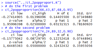
Once this function is defined, we can load it and use it to solve the two problems presented above via commands such as

source("../ci_2popproport.R")
# do the first problem
ci_2popproportion(66,43,87,68,0.95)
# do the second problem
ci_2popproportion(74,24,89,32,0.90)

which produce the results shown in Figure 3.

Figure 3

As expected, the result of the function call shown in Figure 3 gives us all the information that we so carefully constructed in the earlier figures.

This is a good place to look at the effect of having larger samples. To do this we will use the command

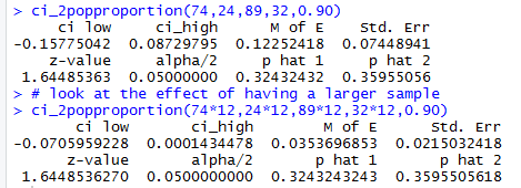
ci_2popproportion(74*12,24*12,89*12,32*12,0.90)

to generate a 90% confidence interval from samples that are 12 times the size of the Case 2 samples but that have exactly 12 times the number of successes in each sample. Thus, the sample proportions will not change even though the samples are much larger. To help look at the effect of having a larger sample Figure 4 first repeats the output of Case 2 and then shows the result of this new command.

Figure 4

Comparing the two results we can see that having that larger sample size reduces the standard error, which reduces the margin of error which results in a narrower confidence interval.

One small addition to this discussion is getting the count of successes in the two samples. We could do this in R via the commands

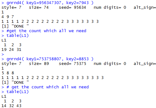
gnrnd4( key1=956347307, key2=7943 )
#get the count which all we need
table(L1)

gnrnd4( key1=753758807, key2=8853 )
# get the count which all we need
table(L1)

Which produce the console view shown in Figure 5.

Figure 5

Clearly, Figure 5 indicates that there were 24 instances of a 2 in Table 1 and 32 instances of a 2 in Table 2.

Hypothesis test on the difference of two proportions

Recall that we are in a situation where we have two populations and each population has a proportion of its members that have some characteristic. We say that p₁ is the proportion of the first population that has the first population characteristic, while p₂ is the proportion of the first population that has the second population characteristic. Here we are interested in running a statistical test of the null hypothesis H₀: p₁ = p₂, which has the equivalent and more useful form H₀: p₁ - p₂ = 0. We will run this test against an alternative hypothesis that is one of

H₁: p₁ - p₂ ≠ 0
H₁: p₁ - p₂ < 0
H₁: p₁ - p₂ > 0

Finally, we will run this test at some specified level of significance.

To do this we want two independent random samples, one from each of the populations. In addition, in order to run this kind of test we need

The samples are big enough to have at least 10 successes and 10 failures in each sample
The samples are small enough so that they represent less than 5% of their respective populations.

In such a situation the distribution of the difference of the proportions will be normal. That means that we can use the standard normal distribution to find either critical values for the stated level of significance or to find the attained significance of a sample statistic.

Remember that in order to make this test we assume that the null hypothesis, H₀: p₁ = p₂, is true. Under that condition our best approximation for the proportion of successes will be

. This is called the pooled sample proportion. Using that pooled sample proportion gives us the standard error defined by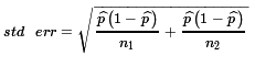

. You may note that this is algebraically equivalent to

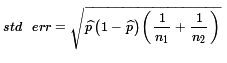, a formula that is often used simply because it is a slightly more efficient computation. With all of this in hand we are ready to look at using either the critical value or the attained significance approach. (It is worth noting that since this is a normal distribution, and since the null hypothesis has the mean of the difference of the proportions be 0, the two approaches will be remarkably similar.)

Case 3: From two very large populations we have taken two samples and found the number of sample members with the specified characteristic in 37 of the 92 items in sample 1 and 28 of the 83 items in sample 2. Our null hypothesis is that the proportion of the members with the specified characteristic in the two populations is the same, i.e., H₀: p₁ - p₂ = 0. Our alternative hypothesis is that the proportion of the members in the first population is greater than the proportion in the second population, i.e., H₁: p₁ > p₂, or its equivalent form H₁: p₁ - p₂ > 0. We want to run this test at the 0.05 significance level.

Critical value approach

For a 5% significance level we need to find the z-value that has 5% of the area under the standard normal curve to the right of that value. We can use a table, a calculator, or the computer to find this. It is approximately z=1.645.

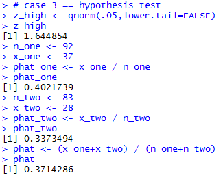
From the data it is interesting to note that = 37/92 ≈0.402 and = 28/83 ≈0.337. However, what we really want is the pooled sample proportion = (37+28)/(92+83) ≈0.3714. These computations can be done in R via the commands

# case 3 == hypothesis test
z_high <- qnorm(.05,lower.tail=FALSE)
z_high
n_one <- 92
x_one <- 37
phat_one <- x_one / n_one
phat_one
n_two <- 83
x_two <- 28
phat_two <- x_two / n_two
phat_two
phat <- (x_one+x_two) / (n_one+n_two)
phat

The result of those commands is given in Figure 6.

Figure 6

Using those results we can find the = 0.0731. Then, the critical value will be the product of our z value with 5% above it times this standard error, or about 1.645*0.0731 ≈ 0.1203. Therefore, we will reject H₀ if the difference in the sample proportions is greater than the critical value 0.1203. However, in this case the difference in the proportions is about 0.0648, a value that is not greater than the critical value and we say that we do not have sufficient evidence to reject H₀ at the 0.05 level of significance.

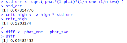
These last calculations can be done in R using

std_err <- sqrt( phat*(1-phat)*(1/n_one +1/n_two) )
std_err
crit_high <- z_high * std_err
crit_high

diff <- phat_one - phat_two
diff

Figure 7 holds the console image of those commands.

Figure 7

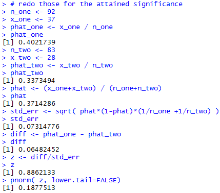
# redo those for the attained significance
n_one <- 92
x_one <- 37
phat_one <- x_one / n_one
phat_one
n_two <- 83
x_two <- 28
phat_two <- x_two / n_two
phat_two
phat <- (x_one+x_two) / (n_one+n_two)
phat
std_err <- sqrt( phat*(1-phat)*(1/n_one +1/n_two) )
std_err
diff <- phat_one - phat_two
diff
z <- diff/std_err
z
pnorm( z, lower.tail=FALSE)

Figure 8 holds the console view of those statements.

Figure 8

Case 4: From two very large populations we have taken two samples and found the number of sample members with the specified characteristic in 54 of the 306 items in sample 1 and 108 of the 422 items in sample 2. Our null hypothesis is that the proportion of the members with the specified characteristic in the two populations is the same, i.e., H₀: p₁ - p₂ = 0. Our alternative hypothesis is that the proportion of the members in the first population is different from the proportion in the second population, i.e., H₁: p₁ ≠ p₂, or its equivalent form H₁: p₁ - p₂ ≠ 0. We want to run this test at the 0.05 significance level.

Critical value approach

Because this is a 2-tail test we need to split that 5% to have 2.5% below and 2.5% above. We need to find the z-value that has 2.5% of the area under the standard normal curve to the right of that value. And we need to find the z-value that has 2.5% of the area under the standard normal curve to the left of that value. Of course, since the standard normal distribution is symmetric these two values will just be additive inverses. We can use a table, a calculator, or the computer to find these values. They are approximately z=1.96 and, of course, z= -1.96.

From the data it is interesting to note that = 54/306 ≈0.1765 and = 108/422 ≈0.2559. However, what we really want is the pooled sample proportion = (54+108)/(306+422) ≈0.2226. These computations can be done in R via the commands

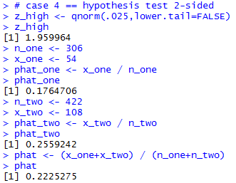
# case 4 == hypothesis test 2-sided
z_high <- qnorm(.025,lower.tail=FALSE)
z_high
n_one <- 306
x_one <- 54
phat_one <- x_one / n_one
phat_one
n_two <- 422
x_two <- 108
phat_two <- x_two / n_two
phat_two
phat <- (x_one+x_two) / (n_one+n_two)
phat

The result of those commands is given in Figure 9.

Figure 9

Using those results we can find the = 0.0312. Then, the critical values will be the product of our z values times this standard error, or about -1.96*0.0312 ≈ -0.0612 and about 1.96*0.0312 ≈ 0.0612. Therefore, we will reject H₀ if the difference in the sample proportions is less than the critical value -0.0612 or greater than the critical value 0.0.0612. In this case the difference in the proportions is about -0.0794, a value that is less than the lower critical value and we say that we reject H₀ at the 0.05 level of significance.

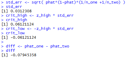
These last calculations can be done in R using

std_err <- sqrt( phat*(1-phat)*(1/n_one +1/n_two) )
std_err
crit_high <- z_high * std_err
crit_high
crit_low <- -z_high * std_err
crit_low

diff <- phat_one - phat_two
diff

Figure 10 holds the console image of those commands.

Figure 10

Attained significance approach

We will do almost all of the above calculations for the attained significance approach. In particular, we compute the sample proportions, the pooled sample proportion, and the standard error. Then we find the difference between the two proportions and divide that difference by the standard error. We have already seen the computation of all those values except for the final division. In this example, that becomes -0.07945/0.0312 ≈ -2.544. This quotient is a z-score and all we need to do is to find the area in the appropriate extreme tail, and then multiply that area by 2. We do this because the alternative hypothesis was H₁: p₁ - p₂ ≠ 0 which means we are looking for the probability of being this or more extreme. We coud be this or more extreme by being in either the lower or the upper tail. Thus, we need to multiply the value here by 2 to account for both tails. In this case, our z-score is negative so we will find the area under the standard normal curve to the left of that value. That value is about 0.00548, giving us about 0.548% of the area to the left of -2.544. When we double that we get about 0.01096 for the attained significance. This is below our stated 0.05 level of significance. Therefore, we reject H₀ at the 0.05 significance level.

Repeating some of the earlier commands, the following R statements compute these values.

# redo those for the attained significance
n_one <- 306
x_one <- 54
phat_one <- x_one / n_one
phat_one
n_two <- 422
x_two <- 108
phat_two <- x_two / n_two
phat_two
phat <- (x_one+x_two) / (n_one+n_two)
phat
std_err <- sqrt( phat*(1-phat)*(1/n_one +1/n_two) )
std_err
diff <- phat_one - phat_two
diff
z <- diff/std_err
z
if ( z > 0 )
  {half_area <- pnorm( z, lower.tail=FALSE)} else
  {half_area <- pnorm( z )}  
half_area
half_area*2

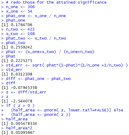
Figure 11 holds the console view of those statements.

Figure 11

As we have noted before, it makes little sense to keep reconstructing these commands. We are far better off if we capture the algorithm in a function. Consider the following possible function definition.

hypoth_2test_prop <- function(
       x_one, n_one, x_two, n_two,
       H1_type, sig_level=0.05)
{ # perform a hypothsis test for the difference of
  # two proportions based on two samples.
  # H0 is that the proportions are equal, i.e.,
  # their difference is 0
  # The alternative hypothesis  is
  #      !=  if H1_type =0
  #      <   if H1_type < 0
  #      >   if H1_type > 0
  # Do the test at sig_level significance.
  phat_one <- x_one / n_one
  phat_two <- x_two / n_two
  phat <- (x_one+x_two) / (n_one+n_two)
  std_err <- sqrt( phat*(1-phat)*(1/n_one +1/n_two) )
  diff <- phat_one - phat_two
  if( H1_type==0)
     { z <- abs( qnorm(sig_level/2))}
  else
     { z <- abs( qnorm(sig_level))}
  to_be_extreme <- z*std_err
  decision <- "Reject"

  if( H1_type < 0 )
     { crit_low <-   - to_be_extreme
       crit_high = "n.a."
       if( diff > crit_low)
         { decision <- "do not reject"}
       attained <- pnorm( diff, mean=0, sd=std_err)
       alt <- "p_1 < p_2"
     }
  else if ( H1_type == 0)
     { crit_low <-  - to_be_extreme
       crit_high <-   to_be_extreme
       if( (crit_low < diff) & (diff < crit_high) )
          { decision <- "do not reject"}

       if( diff < 0 )
         { attained <- 2*pnorm(diff, mean=0, sd=std_err)}
       else
         { attained <- 2*pnorm(diff, mean=0, sd=std_err,
                             lower.tail=FALSE)
         }
       alt <- "p_1 != p_2"
     }
  else
     { crit_low <- "n.a."
       crit_high <-  to_be_extreme
       if( diff < crit_high)
         { decision <- "do not reject"}
       attained <- pnorm(diff, mean=0, sd=std_err,
                         lower.tail=FALSE)
       alt <- "p_1 > p_2"
     }

 result <- c( alt,  n_one, x_one, phat_one,
                    n_two, x_two, phat_two,
                    phat, std_err, z,
                    crit_low, crit_high, diff,
                    attained, decision)
 names(result) <- c("H1:",
                    "n_one","x_one", "phat_one",
                    "n_two","x_two", "phat_two",
                    "pooled", "Std Err", "z extreme",
                    "critical low", "critical high",
                    "difference",
                    "attained", "decision")
 return( result )
}

Once this has been placed in the parent directory under the name hypo_2popproport.R we can load and run that function for the data in Case: 3 via the commands

source("../hypo_2popproport.R")
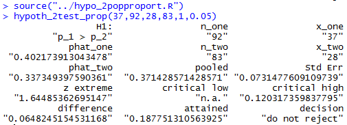
hypoth_2test_prop(37,92,28,83,1,0.05)

The console image of those two commands is shown in Figure 12.

Figure 12

The results shown in Figure 12 are the same as those found above in Figures 6, 7, and 8.

To do Case 4 we use the command

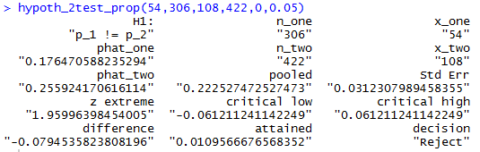
hypoth_2test_prop(54,306,108,422,0,0.05)

to produce the output shown n Figure 13.

Figure 13

The results shown in Figure 123 are the same as those found above in Figures 9, 10, and 11.

To do another example, this one another one-tail test, we use the command

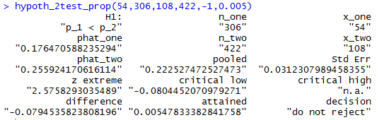
hypoth_2test_prop(54,306,108,422,-1,0.005)

the result of which appears in Figure 14.

Figure 14

Below is a listing of the R commands used in generating this page.

n_one <- 66
x_one <- 43
phat_one <- x_one / n_one
phat_one
n_two <- 87
x_two <- 68
phat_two <- x_two / n_two
phat_two
pe <- phat_one - phat_two
pe
alpha=1-0.95
alphadiv2<-alpha/2
alphadiv2
z <- qnorm(alphadiv2, lower.tail=FALSE)
z
std_err <- sqrt( phat_one*(1-phat_one)/n_one +
                   phat_two*(1-phat_two)/n_two)
std_err
moe <- z*std_err
moe
pe - moe
pe + moe

# second example
n_one <- 74
x_one <- 24
phat_one <- x_one / n_one
phat_one
n_two <- 89
x_two <- 32
phat_two <- x_two / n_two
phat_two
pe <- phat_one - phat_two
pe
alpha=1-0.90
alphadiv2<-alpha/2
alphadiv2
z <- qnorm(alphadiv2, lower.tail=FALSE)
z
std_err <- sqrt( phat_one*(1-phat_one)/n_one +
                   phat_two*(1-phat_two)/n_two)
std_err
moe <- z*std_err
moe
pe - moe
pe + moe

ci_2popproportion <- function(
  n_one, x_one, n_two, x_two, cl=0.95)
{
  phat_one <- x_one / n_one
  phat_two <- x_two / n_two
  pe <- phat_one - phat_two
  alpha=1-cl
  alphadiv2<-alpha/2
  z <- qnorm(alphadiv2, lower.tail=FALSE)
  std_err <- sqrt( phat_one*(1-phat_one)/n_one +
                     phat_two*(1-phat_two)/n_two)
  moe <- z*std_err
  ci_low <- pe - moe
  ci_high <- pe + moe
  result <- c( ci_low, ci_high, moe,
               std_err, z, alphadiv2,
               phat_one, phat_two)
  names( result ) <-
    c("ci low", "ci_high", "M of E",
      "Std. Err", "z-value", "alpha/2",
      "p hat 1", "p hat 2")
  return( result )
}

source("../ci_2popproport.R")
# do the first problem
ci_2popproportion(66,43,87,68,0.95)
# do the second problem
ci_2popproportion(74,24,89,32,0.90)
# look at the effect of having a larger sample
ci_2popproportion(74*12,24*12,89*12,32*12,0.90)


gnrnd4( key1=956347307, key2=7943 )
#get the count which all we need
table(L1)

gnrnd4( key1=753758807, key2=8853 )
# get the count which all we need
table(L1)

# case 3 == hypothesis test
z_high <- qnorm(.05,lower.tail=FALSE)
z_high
n_one <- 92
x_one <- 37
phat_one <- x_one / n_one
phat_one
n_two <- 83
x_two <- 28
phat_two <- x_two / n_two
phat_two
phat <- (x_one+x_two) / (n_one+n_two)
phat

std_err <- sqrt( phat*(1-phat)*(1/n_one +1/n_two) )
std_err
crit_high <- z_high * std_err
crit_high

diff <- phat_one - phat_two
diff

# redo those for the attained significance
n_one <- 92
x_one <- 37
phat_one <- x_one / n_one
phat_one
n_two <- 83
x_two <- 28
phat_two <- x_two / n_two
phat_two
phat <- (x_one+x_two) / (n_one+n_two)
phat
std_err <- sqrt( phat*(1-phat)*(1/n_one +1/n_two) )
std_err
diff <- phat_one - phat_two
diff
z <- diff/std_err
z
pnorm( z, lower.tail=FALSE)


# case 4 == hypothesis test 2-sided
z_high <- qnorm(.025,lower.tail=FALSE)
z_high
n_one <- 306
x_one <- 54
phat_one <- x_one / n_one
phat_one
n_two <- 422
x_two <- 108
phat_two <- x_two / n_two
phat_two
phat <- (x_one+x_two) / (n_one+n_two)
phat

std_err <- sqrt( phat*(1-phat)*(1/n_one +1/n_two) )
std_err
crit_high <- z_high * std_err
crit_high
crit_low <- -z_high * std_err
crit_low

diff <- phat_one - phat_two
diff

# redo those for the attained significance
n_one <- 306
x_one <- 54
phat_one <- x_one / n_one
phat_one
n_two <- 422
x_two <- 108
phat_two <- x_two / n_two
phat_two
phat <- (x_one+x_two) / (n_one+n_two)
phat
std_err <- sqrt( phat*(1-phat)*(1/n_one +1/n_two) )
std_err
diff <- phat_one - phat_two
diff
z <- diff/std_err
z
if ( z > 0 )
{half_area <- pnorm( z, lower.tail=FALSE)} else
{half_area <- pnorm( z )}  
half_area
half_area*2

source("../hypo_2popproport.R")
hypoth_2test_prop(37,92,28,83,1,0.05)
hypoth_2test_prop(54,306,108,422,0,0.05)
hypoth_2test_prop(54,306,108,422,-1,0.005)